Neural Audio Codecs and Discretization: Turning Speech into a Language
Speech Processing & Human–Machine Interaction · Week 6
A language for speech
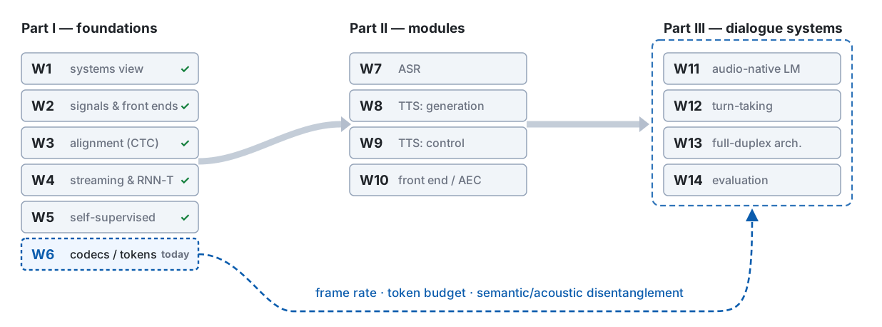
Where we are: week 6 of 14
Last week, in one picture
Week 5 built a target out of nothing — and never rebuilt the waveform. Change the target to the waveform, and three things change with it.
W5 p29 four targets in one row · W5 p55’s last sentence
The problem this week handles, in one picture
A codec invents an alphabet for speech — and every choice in it is a trade among the quantiser, the objective, and the frame rate.
Route: VQ-VAE → residual VQ → listen → two kinds of token → the arithmetic
Notation for today
| Symbol | Meaning |
|---|---|
| \mathbf{x}, f_s, \hat{\mathbf{x}} | waveform (W2’s sampling rate); its reconstruction |
| s_{\text{c}}, f_r = f_s / s_{\text{c}} | the encoder’s total stride; frame rate in Hz (not W4’s s, an ASR subsampling factor) |
| \mathbf{z}_t \in \mathbb{R}^d, \mathbf{q}_t, \hat{\mathbf{z}}_t | latent; quantised latent; the sum of n_q stages (W5’s \mathbf{z}_t, \mathbf{q}_t) |
| V, \mathbf{e}_v, \mathbf{e}^{(i)}_v, k_{t,i} | codebook size and codeword (W5); stage-i codeword; chosen index at stage i |
| N_q, n_q \leq N_q, \mathbf{r}_{t,i} | RVQ stages (not W5’s N, a sample count; not W4’s \mathbf{Q}); stages used; residual after stage i |
| \mathrm{sg}[\cdot], \beta, \mu, c_v, \mathbf{m}_v, n_v | stop-gradient; commitment weight (VQ-VAE); EMA decay (the paper’s \gamma); EMA count and sum; hits of code v in one step |
| \Lambda_j | FSQ levels per dimension (the paper’s L; our L is W2’s window) |
| B, R_{\text{tok}}, \mathcal{L}_{\cdot}, \lambda_{\cdot}, \Phi_j | bitrate; token rate; losses and weights; discriminator j (not D — W1’s delays) |
\log_2 for bits, \ln otherwise · vectors bold, scalars italic, functions upright
Five things to leave with today
- The VQ-VAE loss has three terms and each moves one group of parameters. Straight-through copies a gradient from \mathbf{q}_t to \mathbf{z}_t — biased by the gap \lVert \mathbf{z}_t - \mathbf{e}_{k_t} \rVert — and the commitment term shrinks that gap. The EMA update is online k-means.
- Residual VQ and its bill: B = f_r N_q \log_2 V; residual energy decays stage by stage, so the first stages buy the most, quantizer dropout makes one model serve many bitrates — and most energy in stage 1 is not the semantics.
- Codebook collapse has two causes and five remedies, and FSQ removes it by construction at the price of a low-dimensional bottleneck.
- Two kinds of token, acoustic and semantic, each missing half; three ways to unify them (distillation, split RVQ, one big codebook) — and why AudioLM stacked them.
- The arithmetic: token rate, 30 minutes of context, decoding steps per second, and a latency floor of 1/f_r — the cell of W1’s budget we fill today.
VQ-VAE: inventing the alphabet
Why discrete: an LM reads an index, not a vector
The decoder never sees \mathbf{z}_t. Everything downstream — W8’s TTS, W11’s LM — sees only the integer matrix N_q \times T.
SoundStream / EnCodec: 75 Hz at 24 kHz, strides (2, 4, 5, 8) · Mimi: 12.5 Hz
The three-term loss, and which parameters each term moves
\mathcal{L} = \underbrace{\mathcal{L}_{\text{rec}}(\mathbf{x}, \hat{\mathbf{x}})}_{\text{decoder; encoder via straight-through}} + \underbrace{\lVert \mathrm{sg}[\mathbf{z}_t] - \mathbf{e}_{k_t} \rVert_2^2}_{\text{codebook only}} + \beta\,\underbrace{\lVert \mathbf{z}_t - \mathrm{sg}[\mathbf{e}_{k_t}] \rVert_2^2}_{\text{encoder only}} \mathbf{q}_t = \mathbf{e}_{k_t},\qquad k_t = \arg\min_v \lVert \mathbf{z}_t - \mathbf{e}_v \rVert_2
van den Oord et al. 2017 §3.2 · \beta = 0.25, insensitive from 0.1 to 2.0
Straight-through: where the bias is, what commitment buys
Same trick as W5, different ending. Gumbel-VQ kept the forward pass soft and annealed the bias away; VQ-VAE’s forward pass is hard, so the bias can only be squeezed — by \beta.
VQ-VAE §3.2: without it the encoder output “can grow arbitrarily” · W5 p17
The EMA codebook update is online k-means
c_v^{(\tau)} = \mu\, c_v^{(\tau-1)} + (1-\mu)\, n_v^{(\tau)},\qquad \mathbf{m}_v^{(\tau)} = \mu\, \mathbf{m}_v^{(\tau-1)} + (1-\mu) \sum_{t:\,k_t = v} \mathbf{z}_t \mathbf{e}_v \leftarrow \mathbf{m}_v / c_v \qquad\text{— a decaying average of every latent assigned to } v
\text{k-means M-step:}\quad \mathbf{e}_v \leftarrow \frac{1}{\lvert \{t : k_t = v\} \rvert} \sum_{t:\,k_t = v} \mathbf{z}_t \qquad\text{— the same mean, over the whole data set}
Replace the codebook loss by this and nothing is lost: the codebook was always doing k-means. \mu \to 1 recovers the batch M-step; W5’s HuBERT ran the same algorithm offline and called the result a teacher. Today it is an alphabet.
VQ-VAE App. A.1, eqs. 6–8 · VQ-VAE-2 §2.1 · “online k-means” is our reading
Misconception 1 — “a bigger codebook is a better codebook”
| what you set | what you get, if nothing is done about it | |
|---|---|---|
| init | V = 1024, d = 1024, random | most codewords start far from the data and are never the nearest neighbour |
| update | the codebook loss, or EMA | moves only the codeword that was chosen — an unchosen code never moves |
| size | a bigger V | more codes that are never chosen; the effective alphabet is the number of codes in use |
| W5’s fix | the diversity loss | needs a soft, contrastive setting to push against; we know of no codec that uses it |
Codebook collapse has two causes: an initialisation outside the data’s support, and an update rule that only touches winners. Capacity is the alphabet you use, not V.
DAC §3.2: 8-dim \ell_2 lookups “significantly improve codebook usage” · W5 p19
Before Demo 3: dead codes you can see
| Why | The last slide named two causes of collapse — a codebook initialised outside the data, and an update that only moves the chosen code — and the slide before it claimed EMA is online k-means. In two dimensions all of this is visible. |
| What runs | Pure numpy, a terminal and one plot window. Four Gaussian clusters inside [3, 6]^2, a codebook of V = 16 initialised from \mathcal{N}(\mathbf{0}, \mathbf{I}) — deliberately outside the data. Five ways to train it, 200 steps each: gradient on the codebook loss; EMA; k-means initialisation; dead-code reset; FSQ with \Lambda = (4, 4). Each prints how many codes are used and the quantisation error. |
| Watch for | Whether EMA alone revives any code. Where the used codes sit relative to the dashed data box. What FSQ does without any codebook at all. |
Demo 3 · code: demos/w06_d3_dead_codes · numpy only, CPU
Demo 3 — sixteen codes, four clusters, five ways to train
Demo 3. Before the panels appear: the random-init codebook uses 2 of 16 codes with gradient updates. Switch to EMA — how many does it use?
Demo 3 · demos/w06_d3_dead_codes · seed 20261017 · numbers: w06-data.json
Five remedies in one row
| remedy | what it fixes | source |
|---|---|---|
| EMA update | gradient noise on the codebook — not collapse (Demo 3, panel 2) | VQ-VAE App. A.1; VQ-VAE-2 |
| k-means initialisation | the first cause: start every code inside the data (first batch) | SoundStream §III-C; Łańcucki et al. 2020 |
| dead-code reset | the second cause: a code unassigned for several batches is replaced by a random input frame of the current batch | Jukebox; SoundStream §III-C |
| low-dim, \ell_2-normalised lookup | far-away codes: in 8 dimensions with unit norm the nearest neighbour is a cosine, and no code is “too far” | ViT-VQGAN §3.2 (32 / 8-d); DAC §3.2 |
| FSQ | removes the codebook, hence the problem — at a price (next slide) | Mentzer et al., ICLR 2024 |
all five act on the quantiser freedom · the objective and the frame rate come next
FSQ: no codebook, no collapse — and what it costs
\hat{z}_j = \mathrm{round}\!\big(\lfloor \Lambda_j / 2 \rfloor \tanh z_j\big),\qquad j = 1, \dots, d,\qquad \text{implicit codebook size } \prod_j \Lambda_j
Low dimension is the remedy, in both DAC and FSQ: DAC looks its codebook up in 8 dimensions; FSQ has none and lives in d \approx \log_3 V to \log_8 V.
Mentzer et al. §4.3, §5.3: 99% usage with no tricks · TAAE: FSQ at 400 / 700 bps
Residual VQ and the acoustic codec recipe
Residual VQ: big letters first, then the corrections
\mathbf{r}_{t,0} = \mathbf{z}_t,\qquad \mathbf{q}_{t,i} = \mathrm{VQ}_i(\mathbf{r}_{t,i-1}),\qquad \mathbf{r}_{t,i} = \mathbf{r}_{t,i-1} - \mathbf{q}_{t,i},\qquad \hat{\mathbf{z}}_t = \sum_{i=1}^{n_q} \mathbf{q}_{t,i},\qquad B = f_r\, N_q \log_2 V
Juang & Gray, ICASSP 1982 · SoundStream §III-C · V^{N_q} codewords, N_q V d parameters
The residual shrinks: making change, and where it fails
R(\mathcal{D}) = \tfrac{1}{2}\log_2\!\big(\sigma^2 / \mathcal{D}\big)\qquad\text{— one more bit per dimension halves the distortion}
measured by Demo 2 (2026-10-18) · Cover & Thomas, Ch. 10, for the Gaussian line
Quantizer dropout: one model, one knob, five bitrates
Because the late residual is nearly noise, dropping the late stages costs little — and a decoder that has seen every truncation can decode any prefix. One model covers 1.5 to 24 kbps.
SoundStream §III-C · EnCodec §3.2: codebooks a multiple of 4 · DAC: p = 0.5
Misconception 2 — “the first codebook carries the semantics”
| what the residual curve shows | what it does not show | |
|---|---|---|
| stage 1 | carries the most energy — the coarse spectral envelope and pitch | that it carries the content |
| later stages | carry less, and the late ones look like noise | that they are “detail” in any linguistic sense |
Most energy \neq the semantics. AudioLM had to put w2v-BERT’s semantic tokens on top of SoundStream’s 12 acoustic stages because the first acoustic stage was not semantic enough; and from semantic tokens alone the speaker was gone — speaker classification 3.2%. “Stage 1 = semantics” becomes true only through distillation (p36).
AudioLM §IV-B, §IV-D Table III · this outline’s own old version got this wrong
SoundStream, EnCodec, DAC: three codecs, one table
| SoundStream (2021) | EnCodec (2022) | DAC (2023) | |
|---|---|---|---|
| f_s, strides, f_r | 24 kHz, (2,4,5,8), 75 Hz | 24 kHz, (2,4,5,8), 75 Hz (48 kHz: 150) | 44.1 kHz, stride 512, 86 Hz |
| N_q, V | RVQ, V = 1024 | up to 32 codebooks, V = 1024 | 9 codebooks, 10 bit (V = 1024) |
| bitrate | 3 kbps and up | 1.5 / 3 / 6 / 12 / 24 kbps | 8 kbps |
| codebook care | k-means init, dead-code reset | EMA (0.99) + dead-code reset, “the same training procedure” as Jukebox / SoundStream | 8-dim \ell_2 lookup, dropout p = 0.5 |
| discriminators | multi-res. waveform + STFT | multi-scale STFT (MS-STFT) | multi-period + multi-band |
| what it added | the recipe | the loss balancer; streamable / non-streamable | codebook usage; multi-scale mel loss |
SoundStream §III · EnCodec §3.1–3.4 · DAC Table 1, §3.2
Why a reconstruction loss is not enough: the recipe
\mathcal{L}_{\text{spec}} = \sum_{\text{scale}} \lVert \log\mathrm{mel}(\mathbf{x}) - \log\mathrm{mel}(\hat{\mathbf{x}}) \rVert_1
\mathcal{L}_{\text{adv}} = \sum_j \mathbb{E}\max\big(0,\, 1 - \Phi_j(\hat{\mathbf{x}})\big),\qquad \mathcal{L}_{\text{feat}} = \sum_j \sum_{\ell} \lVert \Phi_j^{(\ell)}(\mathbf{x}) - \Phi_j^{(\ell)}(\hat{\mathbf{x}}) \rVert_1
\mathcal{L} = \lambda_{\text{spec}}\mathcal{L}_{\text{spec}} + \lambda_{\text{adv}}\mathcal{L}_{\text{adv}} + \lambda_{\text{feat}}\mathcal{L}_{\text{feat}} + \mathcal{L}_{\text{VQ}}\ (+\ \mathcal{L}_{\text{dist}})
SoundStream §III-E · MelGAN · HiFi-GAN · W2 p47: the three reasons a vocoder exists
Misconception 3 — “the discriminator is just for sound quality”
Before the answer: take the discriminators away and train the same codec with \mathcal{L}_{\text{spec}} alone, at the same bitrate. Do the tokens now carry more information or less?
| with the adversary | without it | |
|---|---|---|
| phase, fine structure | the decoder invents them; tokens only condition them | the decoder must reproduce them; tokens must encode them |
| at a fixed bitrate | tokens are more abstract, the output is crisp | bits go to detail, and the output is still over-smoothed (W2) |
| Mimi’s extreme | an experiment with only the feature and discriminator losses: “a remarkable boost in audio quality”, MUSHRA 81.0 vs 58.8 | — |
Moshi §3.3.1, Table 4 · whether the released Mimi is that variant: not stated · W2 p47
Misconception 4 — “neural codecs beat Opus”
| the sentence | what it actually claims | |
|---|---|---|
| SoundStream, abstract | “at 3 kbps outperforms Opus at 12 kbps and approaches EVS at 9.6 kbps” | better quality at a quarter of the bitrate, in their own listening test |
| EnCodec §4.5 | “at 3 kbps reaches better performance on average than Lyra-v2 using 6 kbps and Opus at 12 kbps” | an average across categories; on clean speech, Opus at 12 kbps still beats EnCodec at 3 kbps |
| RFC 6716 §2 | Opus: frames 2.5–60 ms, algorithmic delay 5–65.2 ms | Opus’s edge is delay, compute and a standard — none of which the papers claim to beat |
Neural codecs win on quality per bit at low bitrates. “Which is better” is not a question until the bitrate and the latency budget are named.
SoundStream abstract · EnCodec §4.5 · RFC 6716 is a standard, not a paper
Misconception 5 — “MUSHRA scores compare across papers”
| what differs between two papers’ tables | consequence | |
|---|---|---|
| raters | the listeners, the instructions, the anchors, the reference | the scale is re-anchored every time |
| conditions | the test sentences and the bitrate grid | not the same points |
| baselines | each paper runs its own | SoundStream ran Opus and EVS; EnCodec ran Opus and Lyra-v2 — not each other |
Compare codecs only inside one table, or on one shared benchmark — Codec-SUPERB, ESPnet-Codec, DASB — that runs them all under the same protocol. The same rule W1 gave for MOS and W5 gave for leaderboards.
Codec-SUPERB, Findings of ACL 2024 · ESPnet-Codec, SLT 2024 · DASB, TMLR 2026
Hearing the alphabet
Before Demo 1: adding the letters back, one stage at a time
| Why | Every claim so far about what the stages carry — energy first, detail later, content only through distillation — can be heard. Reconstruct the same sentence with more and more stages, and with stage 1 alone. |
| What runs | Three codecs through transformers: Mimi at n_q = 1, 2, 4, 8; EnCodec 24 kHz at 1.5 / 3 / 6 / 12 / 24 kbps; DAC at n_q = 1, 2, 4, 8. Two inputs: the W3 LibriSpeech sentence, and one Mandarin sentence recorded by me. One key per setting; the screen shows f_r, n_q, B and the reconstruction’s log-mel. |
| Watch for | With Mimi’s stage 1 alone: is the content intelligible, and what happens to the voice? For the Mandarin sentence: are the four tones still there? |
Demo 1 · code: demos/w06_d1_layer_listen · inference only · my recording is not published
Demo 1 — Mimi 1 / 2 / 4 / 8, EnCodec 2 … 32, DAC: listen
Demo 1. Before playing: Mimi with stage 1 only, at 137 bps. What do you expect to hear?
| setting | f_r | n_q | B | what we heard (rehearsal) |
|---|---|---|---|---|
| Mimi, 1 / 2 / 4 / 8 | 12.5 Hz | 1 / 2 / 4 / 8 | 0.14 / 0.28 / 0.55 / 1.1 kbps | stage 1: neither words nor voice (prediction failed); back by stage 8 |
| EnCodec 24 kHz | 75 Hz | 2 / 4 / 8 / 16 / 32 | 1.5 / 3 / 6 / 12 / 24 kbps | 1.5 kbps: words and voice clearer than Mimi stage 1 — tenfold bitrate wins |
| DAC 24 kHz, 1 / 2 / 4 / 8 | 75 Hz | 1 / 2 / 4 / 8 | 0.75 / 1.5 / 3 / 6 kbps | 750 bps: also clearer than Mimi stage 1 |
Demo 1 · demos/w06_d1_layer_listen · B = f_r n_q \log_2 V · last column: rehearsal 2026-10-19, one listener
Demo 1 — stage 1 only, in Mandarin: is the tone still there?
Demo 1, second input. Four tones, stage 1 only. Can you still tell 媽 / 麻 / 馬 / 罵 apart? Write down yes or no before it plays.
| prediction from the design | what we heard (rehearsal) | F_0 track | |
|---|---|---|---|
| Mimi, n_q = 1 | tone flattened: W5’s units carry little F_0, and distillation carries that over | flattened — the four tones could not be told apart, and the words went with them | RMSE 57 Hz, voicing agreement 0.49 |
| Mimi, n_q = 8 | tone back, carried by stages 2–8 | tones back | RMSE 5.4 Hz, 0.86 |
| EnCodec, 1.5 kbps | tone kept: pitch is where the energy is | tones kept | RMSE 23 Hz, 0.86 |
F_0 is a physical quantity, pitch is a percept (W2 p51): the plot is a reference, the ear is the judge — and whatever we hear, we say it out loud.
prediction from the design · heard: rehearsal 2026-10-19, one sentence, one listener · W2 p51, p57 · W5 p44 · unit-level evidence: p40
Before Demo 2: what the letters look like
| Why | We have heard what the stages carry; now look at the tokens themselves. Three things on the slides so far were schematic — the residual curve (p20), “stage 1 is the most language-like”, and how many codes are actually used — and all three can be measured on real codecs. |
| What runs | The same sentence through Mimi, EnCodec and DAC: the N_q \times T matrix printed in the terminal. Then, on the W5 dev-clean subset (40 speakers × 10 sentences, cached): per stage, the number of codes used and the unigram entropy over \log_2 V; the residual-energy curve \mathbb{E}\lVert \mathbf{r}_{t,i} \rVert^2 / \mathbb{E}\lVert \mathbf{z}_t \rVert^2; and, for stage 1, the bigram conditional entropy against the unigram one. |
| Watch for | Which stage has the longest runs of repeated tokens. Whether the usage and entropy ratios fall with the stage — and what that says about the late residual. Where Mimi’s semantic path sits relative to its acoustic path. |
Demo 2 · code: demos/w06_d2_token_matrix · the arithmetic half comes at p42
Demo 2 — token matrix, codebook usage, residual curve
Demo 2. Before the numbers: EnCodec has 8 stages of 1024 codes at 6 kbps. Guess the usage ratio of stage 1 and of stage 8.
| codes used / V, stage 1 / 2 / 4 / 8 / 32 | H_1 / \log_2 V, stage 1 / 2 / 4 / 8 / 32 | residual energy after stage 1 / 2 / 4 / N_q | H_2 / H_1, stage 1 | |
|---|---|---|---|---|
| Mimi (S + 31 RVQ in the weights) | 0.71 · 0.82 · 0.96 · 0.98 · 0.92 | 0.90 · 0.89 · 0.91 · 0.92 · 0.94 | S 0.36 · A 0.17 / 0.13 / 0.09 / 0.01 | 0.36 (S), 0.46 (A1) |
| EnCodec 24 kHz, 32 stages | 0.78 · 0.95 · 0.98 · 0.90 · 0.50 | 0.78 · 0.85 · 0.86 · 0.86 · 0.85 | 0.03 / 0.03 / 0.02 / 0.001 | 0.67 |
| DAC 24 kHz, 32 stages | 0.94 · 1.00 · 1.00 · 1.00 · 1.00 | 0.78 · 0.92 · 0.98 · 0.99 · 1.00 | 0.67 / 0.60 / 0.49 / 0.72 (min 0.40 at 9) | 0.80 |
Demo 2 · demos/w06_d2_token_matrix · dev-clean 40 × 10 · measured 2026-10-18
Two kinds of token
Predicted and reconstructed: two tokens, each missing half
Acoustic tokens can rebuild the voice but entangle who, where and what; semantic tokens keep what and lose the voice. Every tokenizer since 2023 asks whether one tokenizer can do both.
W5 p44 · AudioLM, TASLP 2023 · the alphabet’s second failure: letters hold only content
SpeechTokenizer and Mimi: W5’s unit, back inside the codec
Why split: distilling into stage 1 of one RVQ hurts quality — stage 1 is pushed to look like WavLM and the other seven must make up the rest. So Mimi pulls the semantic VQ out and runs the acoustic RVQ beside it.
SpeechTokenizer §3.2, App. E · Moshi §3.3.2 · \mathcal{L}_{\text{dist}}: a cosine distance
Misconception 6 — “a semantic token is a phoneme”
| W5 measured | this week adds | |
|---|---|---|
| the unit | HuBERT units are not phonemes: one id per 20 ms, context-dependent, redundant (p43) | Mimi’s first codebook is a VQ trained to be cosine-close to WavLM, not a phone classifier |
| the probe | purity was measured, not assumed (Demo 2) | on TIMIT, segmental information is not confined to codebook 1, and its tokens correspond to allophones, not phonemes |
Demo 1 did not go as predicted: stage 1 alone kept neither the words nor the voice. “Semantic” names what the codebook was trained towards, not what the ear gets back from it alone — and the tone answer is on p31.
Saloev et al., ICNLSP 2026 (TIMIT) · W5 p41–p43 · “semantic” names a target, not a claim
One codebook, no residual: WavTokenizer, BigCodec, TAAE
| WavTokenizer (ICLR 2025) | BigCodec (2024, preprint) | TAAE (ICLR 2025) | |
|---|---|---|---|
| quantiser | one codebook, V = 4096 | one codebook, V = 8192 | FSQ bottleneck |
| rate | 40 or 75 tokens / s at 24 kHz | 1.04 kbps at 16 kHz | 400 / 700 bps at 16 kHz |
| bitrate at 75 Hz | 0.9 kbps | — | — |
| how usage is kept | k-means initialisation | a low-dimensional VQ | no codebook |
| decoder | iSTFT (Vocos) with attention | — | a Transformer codec |
The third answer: make the one codebook big and the frame rate low, so a time step is one token and the LM needs no depth transformer. The cost is paid by the decoder — and by everything a single code must now carry.
Ji et al. · Xin et al. · Parker et al. · Vocos, ICLR 2024 · other frame rates are derived
2026: letters that do not align — dynamic frame rates
| the failure of the alphabet metaphor | the 2026 answer | |
|---|---|---|
| a fixed grid | one token every 80 ms, whether that holds half a syllable or a pause | FlexiCodec (ICLR 2026): merge semantically similar frames; 3–12.5 Hz controllable at inference |
| a fixed rate | for a signal whose information rate is not fixed | CodecSlime (ICASSP 2026): a dynamic-frame-rate plug-in; an 80 Hz backbone run at 40 Hz |
| no alignment | letters that align to nothing linguistic | DyCAST (2026, preprint): tokens roughly aligned to characters, 6–18 Hz |
| “lower is worse” | the quality cliff at 6.25 Hz | Gichamba & Busogi (Interspeech 2026): it comes from the training setup — too few tokens per fixed-length clip — not from the rate |
Li et al. · Wang et al. · Della Libera et al. · Gichamba & Busogi · all 2026
Tone: evidence at the unit level, a blank at the codec level
Before the answer: distil WavLM into the first codebook. Where does lexical tone go?
At the unit level this is measured; at the codec level it is a prediction — and p31 is where we listened. For Mandarin, Taiwanese and Hakka, a token that drops tone drops the word.
Osakuade & King, Speech Prosody 2026 · Saloev et al. 2026 · W2 p57 · W5 p44
The arithmetic
Demo 2 — the bill: token rate, context, steps, and the floor
Demo 2, second half. A 30-minute conversation. Before the table: how many Mimi tokens — and how many text tokens?
| f_r | N_q | R_{\text{tok}} = f_r N_q | context, 30 min | steps / s, flatten | steps / s, RQ-Transformer | 1/f_r | |
|---|---|---|---|---|---|---|---|
| EnCodec 24 kHz, 6 kbps | 75 Hz | 8 | 600 /s | 1.08 M | 600 | 75 | 13 ms |
| SpeechTokenizer | 50 Hz | 8 | 400 /s | 720 k | 400 | 50 | 20 ms |
| Mimi | 12.5 Hz | 8 | 100 /s | 180 k | 100 | 12.5 | 80 ms |
| text (Gemma 4 tokenizer) | — | — | 2.8 /s | 5.1 k | 2.8 | — | — |
Every column is a function of the three freedoms. Speech tokens outnumber text tokens by one to two orders of magnitude — the other half of W11’s modality gap — and the floor rises exactly as the token rate falls.
Demo 2 · codec rows: arithmetic · text row: one sentence’s rate × 30 min, 2026-10-18
Misconception 7 — “lower bitrate is always better”
Stop and ask: Mimi chose 12.5 Hz for the LM’s sake. Why not 6.25 Hz?
| a lower f_r (or fewer stages) buys | and costs | |
|---|---|---|
| tokens | fewer per second, shorter context, fewer decoding steps | intelligibility and quality: one 80 ms frame may hold a whole short syllable, which one codebook cannot carry alone |
| latency | a cheaper LM | a higher floor 1/f_r: 80 ms at 12.5 Hz, 160 ms at 6.25 Hz — before anything else in the budget |
| reaction | — | coarser: W13’s model decides once per frame |
Three goals pull against each other — feed the LM, keep the voice, react fast — and that conflict is why split RVQ and semantic / acoustic streams exist at all.
Moshi §3.3.1 · Gichamba & Busogi 2026 on the 6.25 Hz cliff · the course’s misconception list
Misconception 8 — “frame rate is an implementation detail”
D_{\text{codec}} \geq 1/f_r + \text{lookahead}
Frame rate is a first-order design choice — context, step count, latency floor and reaction granularity, all at once. Mimi chose it for the LM, not for the signal.
arithmetic (w06-data.json) · W2: the hop · W4 / W5: the stride · W6: somebody chose
Misconception 9 — “a good PESQ makes a good LM input”
| reconstruction metrics | LM-friendliness | |
|---|---|---|
| what is measured | the decoder’s output: PESQ, ViSQOL, MUSHRA, UTMOS | the token sequence: its entropy, long-range structure, drift across speakers |
| so | a high-fidelity codec can score top here | and still give tokens that are high-entropy and weakly structured — hard to model |
Benchmarks that measure the two separately exist for this reason: Codec-SUPERB and DASB report reconstruction and downstream tasks apart; DASB’s abstract: “semantic tokens generally outperform acoustic tokens, but a gap remains between discrete tokens and continuous features.” Park et al. measure the tokens’ own language statistics — Zipf, Heaps, entropy — and their correlation with WER and UTMOS.
Codec-SUPERB 2024 · DASB, TMLR 2026 (check §5 before class) · Park et al., ASRU 2025
Misconception 10 — “a codec token is like a text token”
| text token | codec token | |
|---|---|---|
| rate | ~2–3 per second of speech, read aloud | 10–100× more: 100 to 600 per second |
| per step | one token | N_q tokens — and the LM must decide how to order them |
| dependence | independent symbols | stage i is the residual of stages 1 \dots i-1: dependent by construction |
| drift | the same word is the same token for everyone | the distribution drifts with speaker, room and microphone |
Four differences, and the next two Parts are built on them: W11’s modality gap comes from the first and the last; W13’s multi-stream, RQ-Transformer and delay-pattern architectures are three answers to the second and third.
W11 modality gap · W13: RQ-Transformer (Lee et al. 2022), delay pattern (MusicGen), Moshi
Back to the three axes
Representation: the rightmost slot, and a chosen clock
| W2’s trio | who decided the frame rate | what the representation is |
|---|---|---|
| log-mel (W2) | the hop: 10 ms, 100 Hz | a filterbank, fixed by hand |
| SSL feature (W5) | the CNN stride: 20 ms, 50 Hz | thirteen layers to choose from; a unit that is not a phoneme |
| discrete token (W6) | a design choice: 75 Hz for quality, 12.5 Hz for the LM | an integer matrix N_q \times T; what it carries depends on the objective |
The rightmost slot is filled — and for the first time the clock was chosen, not inherited. W5’s unit came back as the first codebook; the other seven carry what it left out.
W2 p62 · W5 p52 · Mimi: 12.5 Hz for the LM’s sequence length, Moshi §3.3.1
Latency: the cell in W1’s budget, filled in
A codec adds at least one frame: 1/f_r plus any encoder lookahead. A causal codec drives the lookahead to zero at a price in quality — and the frame is also how often a full-duplex model may change its mind.
W1 p31 · W4 p20 D_{\text{alg}} · EnCodec streamable vs not · Mimi: causal, 80 ms frame
The three axes, and supervision’s second answer
| Axis | What we now know |
|---|---|
| Representation | W2’s rightmost slot is filled: an integer matrix N_q \times T, a frame rate that was chosen, content that follows the objective; W5’s unit returns as a distilled first codebook. |
| Latency | At least one frame, 1/f_r, plus lookahead; causal codecs trade quality for zero lookahead; the frame rate is W13’s reaction granularity. |
| Supervision | Still no labels, but a new target — the waveform plus an adversary — and a teacher: W5’s trained model, distilled in. The answer to “where does the supervision come from” changes a second time. |
Three freedoms that constrain each other; two causes and five remedies; two tokens that each miss half; and a bill — token rate, context, steps, a floor of 1/f_r — every later week has to pay.
Reading, and next week
Read this week
- Zeghidour et al., SoundStream, IEEE/ACM TASLP 2022 — §III for the recipe (RVQ, quantizer dropout, k-means init and dead-code reset, the three losses); the abstract’s sentence about Opus, read with p26 in mind
- Défossez et al., Moshi, 2024 (a technical report) — §3.3 only: Mimi — the split RVQ, the WavLM distillation, 12.5 Hz; keep §3.4 and §5 for W13
- van den Oord et al., Neural Discrete Representation Learning, NeurIPS 2017 — §3.2 and Appendix A.1: the three terms and the EMA update you derived today
If one thing today was new to you, make it this one
- Mentzer et al., Finite Scalar Quantization: VQ-VAE Made Simple, ICLR 2024 — §3 and Table 1: a quantiser with no codebook at all
Next week — ASR: three paradigms, streaming, and the LLM turn
Back to a world with transcripts. The encoder is W5’s; the input may be W2’s log-mel or today’s tokens; and the three alignments of W3–W4 become three products. Every latency number from W1 and today comes due.