Self-Supervised Representation Learning: Where Speech Foundation Models Come From
Speech Processing & Human–Machine Interaction · Week 5
No transcript, and a hole to fill
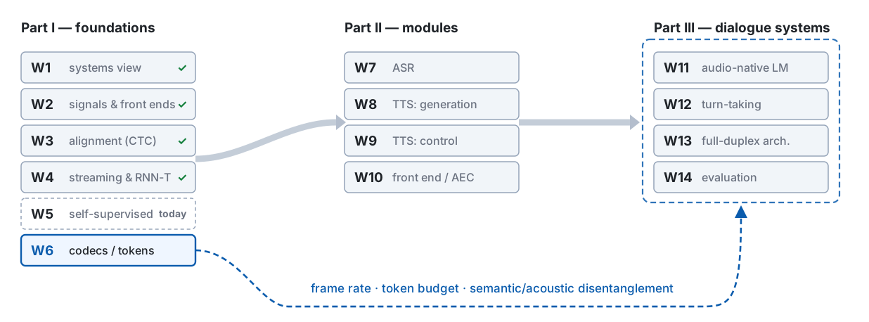
Where we are: week 5 of 14
Last week, in one picture
Week 4 opened the box. It never said where the box’s ability comes from — and every loss it used read a transcript.
W4 p5 the box · p20 D_{\text{alg}} · p54 three alignments, three losses
The problem this week handles, in one picture
One pipeline, one question: what is the answer for the masked frame — and who wrote it down?
Route: contrast → a teacher → layers → units \neq phones → reading a comparison
Notation for today
| Symbol | Meaning |
|---|---|
| \mathbf{x}, \Delta, s | waveform; W2’s hop (10 ms); subsampling (W4). One SSL frame is s\Delta = 20 ms, s = 2 |
| \mathbf{z}_t \in \mathbb{R}^d, \mathbf{c}_t, \mathbf{q}_t | CNN latent; Transformer output (context); quantised latent |
| G, V, \mathbf{e}_{g,v}; \mathbf{e}_k | codebook groups, entries per group, codeword; HuBERT’s unit embedding |
| k_t \in \{1, \dots, K\}, K | cluster id and cluster count (not W4’s u, a lattice index) |
| M, \tilde{\mathbf{X}} | masked positions; the masked input |
| \mathcal{Z} (\mathcal{Z}_t), N = \lvert\mathcal{Z}\rvert, \mathrm{sim}, \kappa, \tau | InfoNCE sample set (one per masked step); cosine; contrastive temperature; Gumbel temperature |
| l = 0, \dots, n_{\text{layer}}, \mathbf{h}^{(l)}_t, \mathbf{w} = \mathrm{softmax}(\boldsymbol{\theta}) | layer index (0 = CNN output), its output, SUPERB’s layer weights |
| I(\cdot\,;\cdot), H(\cdot), \mathcal{L}_m, \mathcal{L}_d, \mathcal{L}_N | mutual information, entropy; masked-prediction, diversity, N-sample InfoNCE losses |
Logs are \ln · two temperatures: \kappa divides a similarity, \tau a Gumbel logit
Five things to leave with today
- InfoNCE is a lower bound on mutual information: the best critic is a density ratio; substitute it back and I(\mathbf{z};\mathbf{c}) \geq \ln N - \mathcal{L}_N. The bound can never exceed \ln N — and that decides what negatives can and cannot buy.
- Four ways to build the target — wav2vec 2.0, HuBERT, data2vec, BEST-RQ — and for each: who builds it, does it move, what stops collapse, how it fails.
- Gumbel-softmax with a straight-through gradient, and a diversity loss that is an entropy: the two pieces W6 will reuse under a harsher name, codebook collapse.
- Layers are not a ladder: speaker low, phones in the middle, and a pre-trained top that can turn back toward the input. Which layer is a representation decision; a learned weighted sum tells you some of it.
- How to read an SSL comparison: data size, domain and model size confound every claim; frozen benchmarks favour a kind of model; and HuBERT’s units are not phonemes.
Targets, first kind: contrast
The pipeline every method shares
A learned filterbank on W2’s clock — 25 ms window, 20 ms hop — fixed at pre-training, before any downstream task exists.
wav2vec 2.0 §2, §3.3 · same front end in HuBERT and data2vec · BEST-RQ eats log-mel
CPC: predict the future, against negatives
\mathcal{L}_N = -\mathbb{E}\!\left[\ln \frac{\exp(\mathrm{sim}(\mathbf{c}_t, \mathbf{z}_{t+k})/\kappa)}{\sum_{\tilde{\mathbf{z}} \in \mathcal{Z}} \exp(\mathrm{sim}(\mathbf{c}_t, \tilde{\mathbf{z}})/\kappa)}\right], \qquad \lvert\mathcal{Z}\rvert = N:\ \text{one positive, } N - 1 \text{ negatives}
Oord, Li & Vinyals 2018, eq. 4 · Table 1: phone probe 64.6% vs MFCC 39.7%
InfoNCE bounds mutual information — in two steps
Read it: \mathcal{L}_N \geq 0, so the bound never exceeds \ln N — 100 negatives cannot show more than \ln 101 \approx 4.6 nat.
CPC App. A.1, eq. 6–11 · a proof without the \approx and \geq: Poole et al. 2019
Before Demo 3: InfoNCE on data with a known answer
| Why | The last slide gave two inequalities: I(\mathbf{z};\mathbf{c}) \geq \ln N - \mathcal{L}_N for any critic, and a ceiling at \ln N because \mathcal{L}_N \geq 0. To see how a trained critic actually behaves under them, use data whose mutual information is known. |
| What runs | Pure numpy, a terminal and one plot window. Two 8-dimensional Gaussian vectors with correlation 0.7 in every dimension, so the mutual information has a closed form: 2.69 nat. A critic is trained with InfoNCE at each N = 2, 4, \dots, 1024, and \ln N - \mathcal{L}_N is averaged over 200 held-out batches. |
| Watch for | The estimate against two lines, the truth and \ln N, as N goes from 2 to 1024 — and what each doubling of N buys. |
Demo 3 · code: demos/w05_d3_infonce_bound · numpy only, CPU
Demo 3 — the ceiling at \ln N
Demo 3. Before the curve appears: at N = 8, can the estimate reach the true value?
Demo 3 · demos/w05_d3_infonce_bound recomputes this curve live (seed 20261011) · numbers: w05-data.json
Misconception 1 — “more negatives is always better”
| what the bound says | what happens in practice | |
|---|---|---|
| few negatives | the ceiling \ln N sits below the truth: you cannot see the information you want | the estimate is pinned under the ceiling (Demo 3: N = 8 gives 1.54 against a ceiling of 2.08 and a truth of 2.69) |
| many negatives | the ceiling clears the truth; the bound can tighten | the ceiling rises only as \ln N: one more nat costs e times the negatives; past the truth, more buys only a smaller variance (Demo 3) |
| wav2vec 2.0 | N - 1 = 100 distractors — a ceiling of \ln 101 \approx 4.6 nat | sampled from the same utterance: same speaker, same channel — only content can separate them |
Hard beats many. The negatives decide what the critic is forced to attend to; their number only decides how high the ceiling is.
wav2vec 2.0 §4.2, App. F (whole-batch negatives hurt) · Poole et al. 2019 §2.3
From predicting the future to filling a hole
Two moves from CPC to wav2vec 2.0: predict the masked, not the future — and quantise the target, so the model cannot make the contrast easy by moving both sides.
vq-wav2vec, ICLR 2020 (quantise, then BERT) · wav2vec 2.0, NeurIPS 2020 (one model)
wav2vec 2.0: the model quantises its own target
Gumbel-softmax and the straight-through gradient
\text{forward (hard):}\quad v^{*} = \arg\max_v\,(l_{g,v} + n_{g,v}),\qquad P(v^{*} = v) = \mathrm{softmax}(l_g)_v\quad\text{(Gumbel-max)}
\text{backward (soft):}\quad \hat{p}_{g,v} = \frac{\exp\big((l_{g,v} + n_{g,v})/\tau\big)}{\sum_{v'} \exp\big((l_{g,v'} + n_{g,v'})/\tau\big)},\qquad \frac{\partial\,(\text{one hot})}{\partial l} := \frac{\partial \hat{p}}{\partial l},\qquad \tau\colon 2 \to 0.5
Straight-through is biased by construction — it pretends the quantiser is the identity. W6’s VQ-VAE reuses it.
Jang, Gu & Poole 2017 · Bengio et al. 2013 · wav2vec 2.0 §4.2: G = 2, V = 320, 102{,}400 codes
The diversity loss is an entropy
\mathcal{L}_d = \frac{1}{GV}\sum_{g=1}^{G}\big(-H(\bar{p}_g)\big) = \frac{1}{GV}\sum_{g=1}^{G}\sum_{v=1}^{V}\bar{p}_{g,v}\ln\bar{p}_{g,v}
\bar{p}_{g,v} is the batch mean of \mathrm{softmax}(l_g)_v over the raw logits — no Gumbel noise, no temperature (wav2vec 2.0 §3.2).
wav2vec 2.0 eq. 4 · \mathcal{L} = \mathcal{L}_m + \alpha\mathcal{L}_d, \alpha = 0.1 · W6: the same disease, no contrast to help
Misconception 2 — “no negatives means collapse”
Collapse is a property of online targets, not of “non-contrastive”. A fixed target cannot collapse and needs no negatives; a moving target can — with or without them.
The whole loss, and where the negatives come from
\mathcal{L} = \mathcal{L}_m + \alpha\,\mathcal{L}_d, \qquad \mathcal{L}_m = -\sum_{t \in M}\ln\frac{\exp(\mathrm{sim}(\mathbf{c}_t, \mathbf{q}_t)/\kappa)}{\sum_{\tilde{\mathbf{q}} \in \mathcal{Z}_t}\exp(\mathrm{sim}(\mathbf{c}_t, \tilde{\mathbf{q}})/\kappa)}
| piece | wav2vec 2.0 BASE | why |
|---|---|---|
| target | \mathbf{q}_t = \mathrm{VQ}(\mathbf{z}_t) at masked t; G = 2, V = 320 | discrete, finite freedom (p15) |
| negatives \mathcal{Z}_t \setminus \{\mathbf{q}_t\} | N - 1 = 100, other masked steps of the same utterance | same speaker, same channel: only content separates them |
| temperatures | \kappa = 0.1 (contrast); \tau\colon 2 \to 0.5 (Gumbel) | two knobs, two jobs |
| masking | spans of 10 steps, start prob. 0.065; \approx 49\% of steps masked | long enough that interpolation fails |
| regulariser | \alpha = 0.1 on \mathcal{L}_d | keep the codebook in use |
Stop. Why must the negatives come from the same utterance? What would the critic learn if they came from other speakers?
wav2vec 2.0 §3.2–3.3, §4.2; App. F
What it costs to build one
64 \times V100 wav2vec 2.0 BASE · 1.6 days · LS-960
128 \times V100 LARGE · 2.3 days (LS-960) · 5.2 days (LV-60k)
32 → 256 GPUs HuBERT BASE → X-LARGE · 250k–400k steps per iteration
| pre-training | today’s demos | |
|---|---|---|
| what runs | tens to hundreds of GPUs, days, 960 h–60k h of audio | inference only: a pre-trained encoder, output_hidden_states=True |
| what it needs | the whole cluster | an M5 Max with 64 GB — and no CUDA |
| what it teaches | — | feasibility is bound to hardware (W1): the first thing this course cannot run even on the instructor’s machine |
Nothing today is training. Not a ten-minute toy either — it would show “it does not finish”, not the phenomenon.
wav2vec 2.0 App. B · HuBERT §IV-C · no demo today is pre-training, by design
Targets, second kind: a teacher
HuBERT: a fixed teacher, then a better one
\mathcal{L}_m = -\sum_{t \in M}\ln p(k_t \mid \tilde{\mathbf{X}}, t), \qquad p(k \mid \tilde{\mathbf{X}}, t) = \frac{\exp(\mathrm{sim}(\mathbf{A}\mathbf{c}_t, \mathbf{e}_k)/\kappa)}{\sum_{k'=1}^{K}\exp(\mathrm{sim}(\mathbf{A}\mathbf{c}_t, \mathbf{e}_{k'})/\kappa)}
Hsu et al., TASLP 2021, eq. 3 (\kappa = 0.1; \tau there) · §IV-C: layer 6, then 9 · arXiv v1 §V-C, Fig. 2: why 6
How good is a teacher? Three purities
HuBERT §IV-E · the MFCC teacher, K = 100: cluster 0.099 · phone 0.335 · PNMI 0.255 (arXiv v1 §V-C)
Misconception 3 — “the k-means must be right to teach”
| teacher (\mathcal{L} = \alpha\mathcal{L}_m + (1-\alpha)\mathcal{L}_u) | \alpha = 1 masked only | \alpha = 0.5 | \alpha = 0 unmasked only |
|---|---|---|---|
| MFCC k-means, K = 100 | 17.86 | 29.57 | 96.37 |
| HuBERT it. 1 layer 6, K = 500 | 11.91 | 13.47 | 23.29 |
| chenone (supervised, for reference) | 10.38 | 9.16 | 9.79 |
dev-other WER after fine-tuning, HuBERT Table V. \mathcal{L}_u is the same loss on the unmasked frames.
“HuBERT relies primarily on the consistency of the unsupervised clustering step rather than the intrinsic quality of the assigned cluster labels.” A bad teacher who answers the same way twice can be learned past — if you only listen to it where you cannot see.
Hsu et al., TASLP 2021, abstract and Table V · the ICASSP 2021 “bad teacher” paper
WavLM: same target, two more tasks, and more data
| HuBERT | WavLM | |
|---|---|---|
| target | k-means ids (it. 2, layer 6 / layer 9) | the same masked prediction of k-means ids |
| input | clean utterance, masked | utterance mixed with noise or another speaker, masked — predict the clean target |
| position | a convolutional relative positional embedding (wav2vec 2.0’s) | adds a gated relative position bias inside attention |
| pre-training data (LARGE) | 60k h Libri-light | 94k h Libri-light + GigaSpeech + VoxPopuli |
| what it buys | content | content, plus a representation that already separates speakers and ignores noise |
Two things changed at once — the auxiliary task and the data. When WavLM wins a benchmark, you cannot tell which one paid. Keep that for p47.
Chen et al., IEEE JSTSP 2022 (abstract: denoising, gated position bias, 60k → 94k h)
data2vec: the teacher is the student, smoothed
\mathbf{y}_t = \frac{1}{K_{\ell}}\sum_{l = n_{\text{layer}} - K_{\ell} + 1}^{n_{\text{layer}}} \mathrm{IN}\big(\mathbf{h}^{(l),\,\text{teacher}}_t\big),\qquad K_{\ell} = 8\colon\ \text{continuous, contextualised, moving}
\boldsymbol{\theta}_{\text{teacher}} \leftarrow \tau_{\text{ema}}\,\boldsymbol{\theta}_{\text{teacher}} + (1 - \tau_{\text{ema}})\,\boldsymbol{\theta}_{\text{student}},\qquad \tau_{\text{ema}}\colon 0.999 \to 0.9999
Baevski et al. 2022 §4.2 · BASE: K_{\ell} = 8, instance norm, L2 at t \in M · \tau_{\text{ema}} rises over 30k updates, then fixed
BEST-RQ: a teacher that knows nothing
A target has to be consistent, not meaningful. The quantiser is frozen noise; what the encoder learns is to predict that noise from context — the same job HuBERT’s student had, with a teacher who knows even less.
Chiu et al., ICML 2022 · codebook 8192 \times 16 · a streaming variant is evaluated (§4)
Four targets in one row
Who builds the target and whether it moves decide three things at once: can it collapse, does it need negatives, can it be iterated. The objective’s name — contrastive, predictive — is downstream of that.
Mohamed et al. 2022 sort by objective; today sorts by target
Misconception 4 — “self-supervised means no labels”
| stage | labels? | what SSL changed |
|---|---|---|
| pre-training | none — but HuBERT’s k_t are pseudo-labels from a teacher a human designed | the target is built, not annotated |
| fine-tuning | yes: 10 min, 1 h, 10 h, 100 h, 960 h | the marginal value of a labelled hour — wav2vec 2.0’s abstract sells ten minutes |
| evaluation | yes, always — WER needs a transcript, purity needs phones, a probe needs speakers | nothing |
SSL moved the labels from the loss to the fine-tuning and the evaluation. It bent the curve of “what an hour of labels buys”; it did not remove the hour.
wav2vec 2.0 Table 1 (10 min → 960 h) · “pseudo-labels” is our word; HuBERT says “cluster assignments”
Layers
Before Demo 1: what does each layer know?
| Why | An SSL encoder gives thirteen representations, not one: the CNN output and twelve blocks. Which layer holds the speaker, which holds the phones, and which still resembles the input decides which layer a downstream task should read. |
| What runs | HuBERT-base, then wav2vec 2.0 base, pre-trained and not fine-tuned, on 400 dev-clean utterances from 40 speakers. For every layer, three numbers: a linear speaker probe, a linear phone probe (labels from MFA forced alignment), and PWCCA with layer 0. Probes and PWCCA are plain numpy; the curves appear point by point. |
| Watch for | If the last layer were the best for everything, all three curves would climb to the top. Watch where each one peaks, and whether any of them peaks at the top. |
Demo 1 · code: demos/w05_d1_layer_probe · torch 2.14.0, transformers 5.17.0
Demo 1 — three curves across thirteen layers
Demo 1. Thirteen layers (l = 0 is the CNN), three numbers each. Before the curves appear: which layer wins each?
| speaker probe: low peak · min · top | phone probe: peak · top | CCA with layer 0: min / top | |
|---|---|---|---|
| HuBERT-base | 2 (0.94) · 8 (0.39) · 0.78 | 11 (0.81) · 0.80 | 0.30 (l9) / 0.36 |
| wav2vec 2.0 base | 2 (0.89) · 8 (0.54) · 0.94 | 9 (0.80) · 0.56 | 0.21 (l7) / 0.29 |
Demo 1 · demos/w05_d1_layer_probe · curves are schematic · table: M5 Max 2026-10-11, w05-metrics.json → demo1 (frame-level probes, held-out)
Why the top layers turn back
| wav2vec 2.0 (pre-trained) | HuBERT / WavLM (pre-trained) | any model, fine-tuned for ASR | |
|---|---|---|---|
| the target the top layer serves | \mathbf{q}_t = \mathrm{VQ}(\mathbf{z}_t): local, a function of one CNN frame | k_t: k-means on an intermediate layer of the previous model | characters / phones |
| so the top layer becomes similar to | the CNN output (layer 0) — “as if reconstructing the input” | that intermediate layer | the transcript; the turn-back disappears |
| where phone content peaks | middle layers, then drops | higher layers | top |
A layer looks like whatever it is asked to predict. The top of a pre-trained encoder is shaped by the pre-training target, not by your task — so “the last layer” is a choice someone else made.
Pasad, Chou & Livescu, ASRU 2021 (Fig. 3) · Pasad, Shi & Livescu, ICASSP 2023 (seven models)
Misconception 5 — “the last layer is the best one”
| if your task is… | read… | because… |
|---|---|---|
| speaker verification, emotion | low layers — or the turned-back top (Demo 1) | the information is acoustic and gets diluted upward, then partly comes back with the turn-back |
| phone recognition, ASR with a frozen encoder | middle layers (wav2vec 2.0) · higher (HuBERT) | content needs context, then the top serves the pre-training target |
| anything, with fine-tuning | the top — after fine-tuning reshapes it | the turn-back disappears once the target is yours |
Measure, do not guess. Which layer is a representation decision; it depends on the model’s pre-training target, and a CCA or a linear probe tells you in an afternoon (Demo 1).
Pasad et al. 2023: the best single layer often matches or beats the weighted sum
SUPERB: a learned weighted sum of layers
\mathbf{h}_t = \sum_{l=0}^{n_{\text{layer}}} w_l\,\mathbf{h}^{(l)}_t, \qquad \mathbf{w} = \mathrm{softmax}(\boldsymbol{\theta})
\boldsymbol{\theta} is learned together with the downstream head; the upstream stays frozen.
Yang et al., Interspeech 2021 · Pasad et al. 2023: best single layer beats the sum by 4–9% (ASR)
Misconception 6 — “higher SUPERB score, better encoder”
Stop. The upstream is frozen, the head is light, the input is a learned weighted sum. What kind of model does this protocol favour?
| the protocol’s choice | what it favours | what it penalises |
|---|---|---|
| frozen upstream | information that is already linearly readable | models that need fine-tuning to show what they know |
| light downstream head | the same | tasks whose head must do real work |
| one weighted sum per task | models whose layers specialise cleanly | models with one strong layer and noisy others |
| the leaderboard itself | WavLM — 94k h, denoising task, gated bias: three changes, one score | — |
A benchmark measures a model under a protocol. WavLM’s lead is partly data and partly the auxiliary task; the protocol cannot split them, and neither can you from the score.
The two “partly”s are this course’s judgement, not a paper’s conclusion
ML-SUPERB, Dynamic-SUPERB: the biases move, not vanish
| what changed | what it showed | the bias it kept, or swapped in | |
|---|---|---|---|
| ML-SUPERB (Interspeech 2023) | 143 languages, few-shot and full | multilingual pre-training does not always beat monolingual — “more data” is not a guarantee either | still frozen upstream; language coverage of the pre-training set is now the hidden axis |
| Dynamic-SUPERB (ICASSP 2024) | instruction-tuned tasks, collaborative task pool | models judged by following instructions, not by a probe | favours models trained to follow instructions; the probe bias is traded for a prompt bias |
Changing the benchmark changes which bias you are measuring under. Read the protocol before the row.
Shi et al. 2023 (143 languages; multilingual \neq always better) · Huang et al. 2024
Units are not phones
Before Demo 2: how phone-like are the units?
| Why | HuBERT’s targets are k-means clusters, often called “phone-like units”. Two questions: how well does each teacher’s clustering line up with phones, and what do the units of one real sentence look like under its phone segments? |
| What runs | k-means with K = 100 (numpy) on the frames of Demo 1’s subset, three times: on MFCC (HuBERT’s first teacher), on HuBERT-base layer 6, on layer 9. Each is scored against the MFA phone labels with the paper’s three measures. Then W3’s sentence: words, phone segments, and its units, one 20 ms cell per frame. |
| Watch for | If units were phones, each phone segment would be one unit and unit edges would sit on phone edges. Watch how the three PNMIs order, how many units one phone takes, and whether mister said by four speakers gets the same units. |
Demo 2 · code: demos/w05_d2_units_vs_phones · shares Demo 1’s subset, alignments and caches
Demo 2 — three teachers, three purities, one sentence
Demo 2. Three teachers: MFCC, HuBERT-base layer 6, layer 9. Before the numbers appear: how do the three PNMIs order — and is layer 9 better than layer 6?
| teacher features | phone purity | cluster purity | PNMI |
|---|---|---|---|
| MFCC (39-d) — HuBERT it. 1’s teacher | 0.257 | 0.101 | 0.304 |
| HuBERT-base, layer 6 — it. 2’s teacher | 0.549 | 0.275 | 0.602 |
| HuBERT-base, layer 9 — LARGE’s teacher | 0.542 | 0.278 | 0.583 |
Measured 2026-10-11 on held-out frames of the Demo 1 subset (7,200 test frames, k-means fitted on 16,526). Paper, LibriSpeech 960 h, K = 100 on MFCC: 0.335 / 0.099 / 0.255 — a different setting; compare the direction, not the digits.
Demo 2 · demos/w05_d2_units_vs_phones · K = 100, numpy k-means · phone labels: the MFA alignments of Demo 1 · → w05-metrics.json
A sentence, in phones and in units
One phone, several units; one unit, several contexts; two speakers, about half the runs in common. Demo 2 measures it: 2.6 units per phone, unit edges on phone edges at chance level, mister across four speakers sharing half its runs (MFCC: a quarter).
schematic (hand-written ids) · Demo 2 key 2 draws it with real units · phone boundaries from the MFA alignment, not CTC spikes
Misconception 7 — “a discrete unit is a phoneme”
| phoneme | HuBERT unit |
|---|---|
| a linguistic category: ~39 for English, defined by contrast between words | a k-means cell: K = 50–500, defined by distance in a layer’s feature space |
| one symbol per segment, variable duration | one id per 20 ms frame — finer, many ids per segment |
| context-independent by definition | context-dependent: the same phoneme lands on different ids |
| no redundancy by construction | redundant ids (Sicherman & Adi 2023) |
| carries no speaker, no F0 | speaker reduced, not gone; F0 largely absent — by design, not by accident (next slide) |
Units correlate strongly with phonemes and that is exactly what makes the confusion tempting. They are a quantised, contextual, redundant code — the raw material of W6’s tokens and W11’s unit LM, not a phonetic transcription.
Lakhotia et al., TACL 2021 (GSLM) · Sicherman & Adi, ICASSP 2023 · Polyak et al., Interspeech 2021
Where speaker and F0 went: three streams
For English, splitting content / prosody / speaker is a sensible disentanglement. For Mandarin, Taiwanese and Hakka, tone is lexical content and lives in the F0 stream — the units may carry less of the word than they do in English. A prediction, not a measurement; W6 and W11 return to it.
Polyak et al., Interspeech 2021 (abstract: content, prosody, speaker extracted separately)
Reading a comparison
Three confounders under every leaderboard
Match all three before reading the row — and multilingual does not even guarantee a win (ML-SUPERB).
wav2vec 2.0 Table 1 · Robust wav2vec 2.0, Interspeech 2021 · ML-SUPERB, Interspeech 2023
Misconception 8 — “A beats B, so A’s architecture wins”
| model | pre-training data | 10 min labels, test-clean / test-other | 100 h labels, test-clean / test-other |
|---|---|---|---|
| wav2vec 2.0 LARGE | LibriSpeech 960 h | 6.8 / 10.8 | 2.3 / 5.0 |
| wav2vec 2.0 LARGE — same architecture | Libri-light 60k h | 4.8 / 8.2 | 2.0 / 4.0 |
WER (%) with a Transformer LM, wav2vec 2.0 Table 1. One row to the next: the objective, the architecture, the fine-tuning recipe are identical.
Before crediting an architecture, line up the pre-training hours, the domain and the size. HuBERT LARGE and WavLM LARGE are 60k-hour-plus models; a comparison with a 960-hour BASE says little about objectives.
Baevski et al., NeurIPS 2020, Table 1 · HuBERT / WavLM LARGE: 60k h / 94k h
Domain shift: pre-train on what you will test on
| mismatch | what the paper varied | what it found (abstract) |
|---|---|---|
| pre-train \neq test | read audiobooks vs conversational / far-field / other corpora, in pre-training, fine-tuning and test | adding unlabelled target-domain data to pre-training “leads to large performance improvements” |
| how much is recovered | — | the gap to in-domain pre-training closes by 66–73 % |
| what this course needs | Part III is conversational speech: overlap, laughter, fillers, far-field | the pre-training set of the encoder you pick is a design decision for W10 and W12 |
The cheapest hour of data you can add is an unlabelled hour from the right domain. This is the supervision axis’s second lesson today: labels moved to fine-tuning, and domain moved into pre-training.
Hsu et al., Robust wav2vec 2.0, Interspeech 2021 — numbers from the abstract
Misconception 9 — “an SSL encoder streams as it is”
| a standard SSL encoder | what streaming needs | the bill (W4’s accounting) | |
|---|---|---|---|
| attention | bidirectional, whole utterance | a causal or chunked mask (W4’s C, m, H) | retrain or fine-tune with the mask; a quality cost (W4 p21–p22) |
| frame rate | s\Delta = 20 ms, fixed by the CNN | W4’s Conformer ran at 40 ms | twice the frames: T doubles, T^2 quadruples, KV cache doubles |
| compute per frame | ~100M (BASE) to ~300M (LARGE) parameters every 20 ms | a term D_{\text{comp}} did not have | measure it (W3 Demo 3’s MPS number is one forward of one short utterance) |
Only BEST-RQ among today’s papers evaluates a streaming variant — pre-trained with a streaming objective, not converted afterwards.
“Pre-trained encoder” does not mean “ready for the budget”. The non-causal box of W4 is the default here — and the 20 ms clock was set before you arrived.
BEST-RQ §4 · W4 p13 (s), p20 (D_{\text{alg}}), p56 (KV cache) · W1 p31 budget
Misconception 10 — “Whisper is self-supervised too”
| this week’s models | Whisper (W4 Demo 3’s model) | |
|---|---|---|
| training signal | none — a target the model or a teacher builds | 680k hours of transcribed audio: weak supervision, but supervision |
| architecture | encoder only; a head is added later | encoder–decoder, trained end-to-end to emit text |
| what it learned | a representation; what it is for is decided downstream | ASR and translation directly |
| how to compare | on a frozen-upstream benchmark, or after fine-tuning | as an ASR system; its encoder can be probed, but it was never trained without text |
Two roads to a speech foundation model: no transcripts and a built target (today), or a great many transcripts (Whisper). W7 puts them side by side; do not file them under one name.
W4 p50 (Whisper cross-attention heads) · W7 compares the two roads
Back to the three axes
Representation: W2’s middle slot, filled in
| W2 / W4 | today | |
|---|---|---|
| the three representations (W2 p62) | log-mel · SSL feature · discrete token — two of them placeholders | the middle one is \mathbf{c}_t or \mathbf{h}^{(l)}_t; the third has a prototype: the k-means unit k_t |
| who decides the frame rate | the hop, then s (W4: a design choice) | the CNN’s stride, chosen at pre-training: 20 ms, before any task exists |
| what the representation carries | whatever the loss asked for | content, strongly; speaker, reduced; F0, largely not — and that is a decision (three streams) |
| which layer | — | a representation decision: speaker low, phones middle, top shaped by the target |
The middle of the trio is not one vector but thirteen, and the choice among them belongs to the representation axis. W6 takes the unit and asks it to reconstruct, not predict.
Latency and supervision: the answer changes
| Axis | What today added | The price, or the lesson |
|---|---|---|
| Latency | a bidirectional encoder as the default; a 20 ms clock set by the CNN; 10^8–3 \times 10^8 parameters per frame | streaming is a retrain, not a switch; T doubles against W4’s 40 ms; a new term in D_{\text{comp}} |
| Supervision | pre-training with no transcript: the target is built by a quantiser, a teacher, an EMA copy, or a random matrix | labels moved to fine-tuning and evaluation; their marginal value changed; domain moved into pre-training (unlabelled target-domain hours) |
W3 and W4 asked “where does the alignment come from”; today asked “where does the target come from” — and the answer “the model builds it” continues into W6’s codecs and W11’s unit language models.
What this week put on the three axes
| Axis | What we now know |
|---|---|
| Representation | The middle of W2’s trio is thirteen layers, not one; the frame rate was fixed at pre-training; the k-means unit is the first discrete token, and not a phoneme. |
| Latency | Bidirectional by default; a 20 ms clock; 10^8 parameters per frame. Streaming is a retrain. |
| Supervision | No transcript: the target is built. Labels moved to fine-tuning and evaluation; domain moved into pre-training. |
A bound that caps at \ln N; four ways to write the answer down; thirteen layers to choose from; a unit that is not a phoneme; and three confounders under every comparison.
Reading, and next week
Read this week
- Mohamed et al., Self-Supervised Speech Representation Learning: A Review, IEEE JSTSP 2022 — the survey; read the taxonomy section, then re-sort it by target as we did today
- Hsu et al., HuBERT, IEEE/ACM TASLP 2021 — §II for the loss, §IV-E for the three purities, Table V for the \alpha ablation you saw
- Baevski et al., wav2vec 2.0, NeurIPS 2020 — §2–3 and Appendix B; look at Table 1 with p47 in mind
If one thing today was new to you, make it this one
- Pasad, Chou & Livescu, Layer-wise Analysis of a Self-supervised Speech Representation Model, ASRU 2021 — Fig. 1 and Fig. 3 are the whole “layers” section in two pictures
Next week — neural audio codecs and discrete tokens
Today’s unit was predicted; next week’s token is reconstructed. What changes when the target is the waveform itself: residual VQ, codebook collapse in its harsher form, bitrate against intelligibility — and why W6 is the hinge of the course.