Sequence Models and Streaming Architectures: Transformer, Conformer, RNN-T

Speech Processing & Human–Machine Interaction · Week 4

Hung-Shin Lee

Two holes, and one constraint

Where we are: week 4 of 14

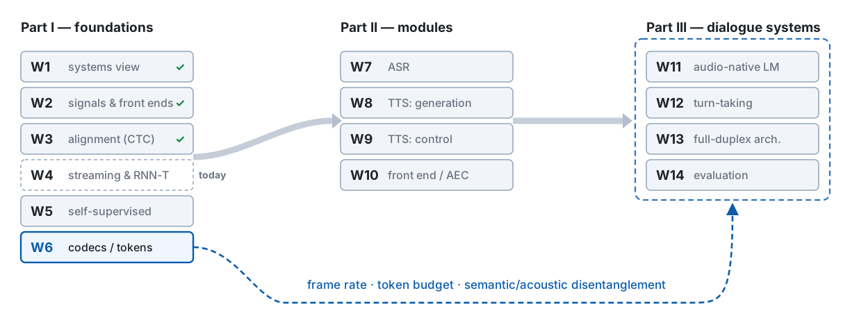
Last week, in one picture

Week 3 gave us a loss and a gradient. It also left two holes: the outputs never see each other, and we never opened the box that makes them.

The problem this week handles, in one picture

Open the box, give the output a memory, meet the third alignment — and through all three: how much of the future may the model see before it answers?

Notation for today

Symbol	Meaning
\mathbf{x}_t, \mathbf{X}, T	W2 frames; T is now the frame count after subsampling
\ell = (\ell_1, \dots, \ell_U), \mathcal{V}, \varnothing, \mathcal{V}' = \mathcal{V} \cup \{\varnothing\}, \mathcal{L}	as in W3: labels, vocabulary, blank, loss
\mathbf{f}_t \in \mathbb{R}^d	encoder output at frame t
\mathbf{g}_u = g(\ell_{1:u}), u = 0, \dots, U	prediction-network output after u labels (\mathbf{g}_0: empty prefix)
\mathbf{z}^{t,u}, \mathbf{y}^{t,u} = \operatorname{softmax}(\mathbf{z}^{t,u}), y^{t,u}_k	joint logits, softmax, one entry — per lattice node
y(t,u) = y^{t,u}_{\ell_{u+1}}, \varnothing(t,u) = y^{t,u}_{\varnothing}	emit the next label / consume a frame (Graves 2012)
\mathbf{Q}, \mathbf{K}, \mathbf{V}, d_k, h, \mathbf{M}, n_{\text{layer}}	attention: projections, head width, head count, mask, depth
\Delta, s, C, H, r_k, m = \sum_k r_k, \alpha	W2 hop; subsampling; chunk and history (W1); right context per layer; lookahead (W1 wrote \ell); chunk-wait coefficient (W1)

Five things to leave with today

1. Attention’s dimension flow and its T \times T score — and the Conformer block: convolution gives the local bias attention lacks; relative positions because chunks make absolute ones meaningless.
2. Two mechanical delays: right context per layer stacks (m = \sum_k r_k); the chunk wait does not (\alpha C). Both are in encoder frames: D_{\text{alg}} = (m + \alpha C)\,s\Delta.
3. The RNN-T in full: the (t, u) lattice, \alpha, \beta, P = \alpha(T,U)\,\varnothing(T,U), and a gradient that reads as occupancy \times softmax - edge posterior — W3’s y - \gamma with one factor in front.
4. A third delay the architecture does not show: emission delay, which the loss can be told to fight (FastEmit).
5. Attention is not alignment, and the state of a Transformer grows with T.

The box: Transformer and Conformer

Attention in one line: three matrices and a T \times T score

\operatorname{Attn}(\mathbf{Q}, \mathbf{K}, \mathbf{V}) \;=\; \operatorname{softmax}\!\left(\frac{\mathbf{Q}\mathbf{K}^{\top}}{\sqrt{d_k}} + \mathbf{M}\right)\mathbf{V}, \qquad \mathbf{Q} = \mathbf{X}\mathbf{W}_Q,\ \mathbf{K} = \mathbf{X}\mathbf{W}_K,\ \mathbf{V} = \mathbf{X}\mathbf{W}_V

Multi-head, and the mask as an addition

Multi-head. h attentions in parallel, each of width d_k = d/h, concatenated and projected once: \operatorname{MHA}(\mathbf{X}) = [\text{head}_1; \dots; \text{head}_h]\,\mathbf{W}_O, \mathbf{W}_O \in \mathbb{R}^{d \times d}. Same cost as one head of width d; h different ways to read the same frame.

The mask is an addition, not a multiplication. M_{ij} \in \{0, -\infty\} is added before the softmax:

M_{ij} = 0 \;\text{(frame } i \text{ may read frame } j), \qquad M_{ij} = -\infty \;\Rightarrow\; e^{-\infty} = 0 \;\text{(it may not)}

Mask	Rule	What it buys
none	M_{ij} = 0	the whole utterance, and the whole wait
causal	M_{ij} = -\infty \iff j > i	zero lookahead, zero chunk wait, large quality cost
chunk + lookahead + history	M_{ij} = 0 \iff j \leq c(i)\,C + R \;\wedge\; i - j \leq H, c(i) = \lceil i / C \rceil	the design space of streaming encoders — next section

Conformer: four modules, one block

Misconception 1 — “the conv module just adds a bit of locality”

Step (each removes one more thing — cumulative)	dev-other	test-other
Conformer (M)	4.4	4.3
- Swish, + ReLU	4.4	4.5
- convolution module	4.8	4.9
- Macaron FFN	5.1	5.0
- relative positional encoding	5.8	5.6

The paper’s own conclusion: “the convolution sub-block is the most important feature.” Read the table as one path from Conformer to Transformer, not as five independent experiments — the last step’s jump is also the step that lands on a vanilla Transformer.

Subsampling: s decides T, and T decides the rest

Two stride-2 convolutions at the front: T_{\text{front}} = 100 frames per second becomes T = T_{\text{front}} / s, s = 4 → one encoder frame every 40 ms.

What s touches	How
attention cost	T^2 shrinks by s^2: 16\times fewer scores per layer at s = 4
W3’s floor T \geq U + r	tighter by s: characters per second vs. 100/s frames per second
every latency term	r_k and C are counted in encoder frames — one frame is s\Delta, not \Delta
the blank	one per encoder frame: this is the clock the RNN-T’s \varnothing advances

W2’s answer to who decides the frame rate was “the hop, times every stride.” s is that stride — the first frame-rate choice that is a design parameter.

Why relative positions: Transformer-XL’s four terms

Absolute positional encoding adds a position vector to each input; the score between i and j then depends on where in the sequence each sits. Transformer-XL rewrites the score so that position enters only as the distance i - j:

A^{\text{rel}}_{ij} \;=\; \underbrace{\mathbf{q}_i^{\top}\mathbf{k}_j}_{\text{(a) content}} \;+\; \underbrace{\mathbf{q}_i^{\top}\mathbf{W}_{R}\,\mathbf{r}_{i-j}}_{\text{(b) content-dependent position}} \;+\; \underbrace{\mathbf{u}^{\top}\mathbf{k}_j}_{\text{(c) global content bias}} \;+\; \underbrace{\mathbf{v}^{\top}\mathbf{W}_{R}\,\mathbf{r}_{i-j}}_{\text{(d) global position bias}}

\mathbf{r}_{i-j} is a sinusoid of the offset; \mathbf{u}, \mathbf{v} are learned and shared across positions.

Under chunks or segment recurrence, a frame’s absolute index inside the current piece is arbitrary: the same acoustic event would get a different representation at the head of a chunk than at its tail. Relative scores are shift-invariant, so the chunking stops leaking into the content.

Making the box causal: four families

Four ways to turn a non-causal encoder into a streaming one

Family	Mechanism	Delay term	Stacks?	Example
causal mask	M_{ij} = -\infty, j > i	none (m = 0, C = 1)	—	cheapest, worst quality
chunk + lookahead	read to the chunk end, +R past it, \leq H back	\alpha C\,s\Delta (chunk) + m\,s\Delta if R is re-read per layer	chunk: no · R: yes	Transformer Transducer; Chen et al. 2021
memory / state carry-over	a compressed summary of past segments replaces H raw frames	none: bounds the history	—	Transformer-XL; Emformer
latency-controlled BLSTM	backward LSTM over a short future window only	the window: m\,s\Delta	no — the window is re-cut per chunk at every layer	Zhang et al. 2016

Only two quantities change: how far right a layer reads, and whether that compounds with depth. The past costs memory, not time.

The mask, drawn: causal, chunk, R, H

Two delays, one picture: what stacks and what does not

The two derivations, one line each

(a) Right context stacks. Layer k’s output at t needs layer k-1’s output up to t + r_k. Apply it n_{\text{layer}} times:

t^{(k)} = t^{(k-1)} + r_k \quad\Longrightarrow\quad t^{(n_{\text{layer}})} = t + \sum_{k=1}^{n_{\text{layer}}} r_k = t + m \qquad\text{(W1 p34, now in encoder frames)}

(b) The chunk wait does not. Claim: if every layer reads only up to the end of the current chunk, then layer n_{\text{layer}}’s output anywhere in chunk c depends on the input only up to the end of chunk c. Induction: true for layer 1 by the mask; if true for layer k-1, then layer k reads layer k-1 only within chunk c, whose values depend on input only up to the end of chunk c. \square

The last frame of the user’s speech lands at position j in its chunk and waits (C - 1 - j) frames: mean \tfrac{C-1}{2}, worst C - 1 — W1’s \alpha \in [\tfrac12, 1], with C - 1 rounded to C.

Two mechanisms, two shapes: a sum over layers and a single shared boundary.

D_{\text{alg}} = (m + \alpha C)\,s\Delta: W1’s formula, with the missing s

D_{\text{alg}} \;=\; \underbrace{m\,s\Delta}_{\text{right context, summed over layers}} \;+\; \underbrace{\alpha\,C\,s\Delta}_{\text{chunk wait, shared by all layers}}, \qquad m = \sum_{k=1}^{n_{\text{layer}}} r_k, \quad \alpha \in [\tfrac12, 1]

W1 wrote \ell\Delta + \alpha C\Delta on the 10 ms grid — correct for a model with no subsampling. The encoder’s frame is s\Delta.

Compute it. r_k = 2 at every layer, n_{\text{layer}} = 12, s = 4, \Delta = 10 ms. Chunk C = 8 encoder frames, \alpha = \tfrac12. How many milliseconds before the first symbol can even be computed?

	encoder frames	ms
m = 12 \times 2	24	960
\alpha C = \tfrac12 \times 8	4	160
D_{\text{alg}} (mean)	28	1120 — worst case 1280

Misconception 2 — “add lookahead to get the quality back”

Raising r_k from 2 to 8 at every layer, with s = 4:

\text{per layer: } 2 \times 40 = 80 \text{ ms} \;\longrightarrow\; 8 \times 40 = 320 \text{ ms} \qquad\text{(not } 20 \to 80\text{: that forgot } s\text{)}

• One layer at r_k = 8 already spends a whole human-scale budget (a few hundred ms, W1).
• Lookahead’s benefit saturates quickly; its cost is linear, per layer, and in s\Delta units.
• The budget is spent at the sum, so the only cheap right context is the kind that does not stack: put it in the chunk, or copy it per segment (Emformer, p23).

Before adding one frame of right context, ask three questions: which layer, times how many layers, times what frame size.

Misconception 3 — “streaming is just a causal mask”

Setting	m	C	D_{\text{alg}}	What you pay
purely causal	0	1	\approx 0	the largest quality loss; every frame answers with no future
chunk only	0	C	\alpha C\,s\Delta	a bounded wait, flat in depth
chunk + per-layer R	n_{\text{layer}} R	C	(n_{\text{layer}} R + \alpha C)\,s\Delta	quality back; latency summed over depth
chunk + copied R (Emformer)	R	C	(R + \alpha C)\,s\Delta	right context once, not per layer

Streaming is a three-number trade-off — m, C, H — not a switch. The causal mask is one corner of that space, and the corner nobody ships.

History: Transformer-XL recurrence, Emformer, LC-BLSTM

Transformer-XL. Layer n of segment \tau + 1 attends to [\,\operatorname{SG}(\mathbf{h}^{\,n-1}_{\tau})\,;\ \mathbf{h}^{\,n-1}_{\tau+1}\,] — the previous segment’s states, stop-gradient, as extra keys and values: history costs memory, not waiting. Emformer. \mathbf{K}^n_i = [\,\mathbf{W}_k \mathbf{M}^n_i,\ \mathbf{K}^n_{L,i},\ \mathbf{W}_k \mathbf{C}^n_i,\ \mathbf{W}_k \mathbf{R}^n_i\,] — memory bank (one vector per past segment, carried over from the lower layer), cached left context, centre chunk, and the hard-copied right context drawn above.

Refill W1’s budget: the encoder row

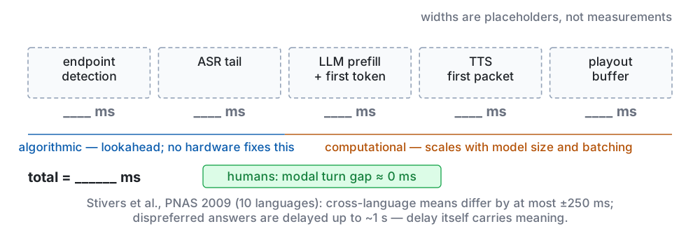
Cell	Fill with	Today’s example
ASR tail (encoder part)	D_{\text{alg}} = (m + \alpha C)\,s\Delta — write the s	1120 ms mean
…and a term W1 did not have	+ emission delay (next section)	measured, not computed

RNN-T: a second axis on the lattice

Three networks, one joint

The prediction network sees only the labels emitted so far. That is where the output dependency CTC gave up comes back — and it comes back without touching the monotonic lattice.

Who sees what, and how often each one runs

	encoder	prediction network	joint network
its job	acoustic evidence	the text so far: an output-side LM	the decision at one node
in → out	\mathbf{X} \to \mathbf{f}_t, one per frame	\ell_{1:u} \to \mathbf{g}_u, one per prefix	(\mathbf{f}_t, \mathbf{g}_u) \to \mathbf{y}^{t,u}
never sees	the labels	the audio	any other node
training	all T frames at once	the gold \ell: \mathbf{g}_0, \dots, \mathbf{g}_U at once	every node: T(U+1) softmaxes
greedy decoding	once per frame	once per emitted label	once per step: T + \hat{U}
in CTC (W3)	the whole model	absent: outputs independent	a softmax per frame

Audio and text meet only in the joint, one node at a time — so the joint alone decides each step: emit a label, or say \varnothing and take the next frame.

One greedy decode, step by step

Right: one joint evaluation and a new frame. Up: one joint evaluation plus a prediction-network step — a cost per label, not per second.

Misconception 4 — “the RNN-T blank is the CTC blank”

	CTC (W3)	RNN-T (today)	W1’s \varnothing
what \varnothing means	this frame emits no new label — a bookkeeping symbol	consume one frame; advance t — a clock	the system is not speaking in this slot
on the lattice	stay in the same row of \ell'	move right one column	—
labels per frame	exactly one symbol of \mathcal{V}'	zero, one, or several, then a blank	—
repeated labels	need a blank between them (\mathcal{B} collapses)	need nothing: emit and emit	—

Same glyph, three semantics. W3 p58 planted this; here it is paid: the RNN-T’s blank is time, and that is exactly what lets labels pile up inside one frame.

The lattice: right is a frame, up is a label

Before Demo 1: the RNN-T lattice, by hand and by program

Why	The CTC lattice had one way to move; this one has two, and emitting does not cost a frame. Count the paths by hand to feel the difference, then check the RNN-T forward recursion against brute force, as in W3.
What runs	A terminal program in the style of W3’s Demo 2 (standard library, fixed seed), used three times: next slide, the paths for “ab” and “aa”, on paper first; at Misconception 5, greedy decoding on a synthetic joint with and without a cap of 5 symbols per frame; after the forward recursion, one random \mathbf{y}^{t,u} through enumeration and through the table.
Expect	Enumeration and forward agree to the last digit; if they do not, the recursion is wrong. Watch the CTC count beside the RNN-T one: can RNN-T have a path where CTC has none? And what does the decoder do once the cap is gone?

Paths: write them out before the program does

Demo 1, part 1. On paper: \ell = \text{ab}, T = 2. List every RNN-T path as a sequence of right / up moves. How many? Then \ell = \text{aa}, T = 1.

\ell	T	RNN-T paths (E = emit, R = blank)	RNN-T count	\binom{T+U-1}{U}	CTC count (W3)
ab	1	E E R	1	1	0
ab	2	E E R R · E R E R · R E E R	3	3	1
ab	3	6 paths	6	6	5
aa	1	E E R	1	1	0
aa	2	3 paths	3	3	0
aa	3	6 paths	6	6	1

Counting paths: \binom{T+U-1}{U}, and no floor on T

\#\,\text{paths} \;=\; \binom{T + U - 1}{U} \qquad\text{vs. CTC: } \lvert \mathcal{B}^{-1}(\ell) \rvert, \text{ which is } 0 \text{ whenever } T < U + r

	CTC	RNN-T
labels per frame	exactly one symbol of \mathcal{V}'	any number, then a blank
repeated labels	a blank must separate them	nothing needed: emit, emit
minimum T	U + r	1
what replaces the floor	—	compute: one more joint evaluation per emit

W3’s floor on the frame rate is gone; in its place a cost per emitted label — the opening TDT exploits by predicting durations too.

Misconception 5 — “RNN-T also needs T \geq U + r”

…and its twin, “an RNN-T emits at most one label per frame.” Both wrong, for the same reason: emitting does not consume a frame. A path may go up as many times as it likes before it goes right; T = 1 already has a path for any \ell.

But every decoder you will meet has a line like

max_symbols_per_step = 5   # stop emitting, force a blank, move on

• That cap is an engineering limit on greedy / beam search — it bounds the number of joint evaluations per frame and prevents a runaway loop of emits.
• It is not a property of the model: the training sum includes paths that emit more than that in one frame.
• Remove the cap (Demo 1, part 3) and watch what a badly calibrated \varnothing(t,u) does.

Forward on the RNN-T lattice

\alpha(t,u) \;=\; \alpha(t-1,u)\,\varnothing(t-1,u) \;+\; \alpha(t,u-1)\,y(t,u-1), \qquad \alpha(1,0) = 1

P(\ell \mid \mathbf{X}) \;=\; \alpha(T,U)\,\varnothing(T,U)

Check the recursion against brute force

Demo 1, part 2. Random \mathbf{y}^{t,u} for \ell = \text{ab}, T = 2. First multiply out the 3 paths and add. Then fill \alpha(t,u) cell by cell. Same number?

	\ell = \text{ab}, T = 2	computed where
uniform y^{t,u}_k = \tfrac13: enumeration = 3 \times 3^{-(T+U)}	0.037037\ldots	w04-data.json
uniform: \alpha(T,U)\,\varnothing(T,U)	0.037037\ldots — equal	w04-data.json
random \mathbf{y}^{t,u} (seed 20261004): enumeration vs. forward	0.0081738\ldots, difference 0.0	w04-data.json
live, your random \mathbf{y}^{t,u}	(read from the screen)	Demo 1, keys 4 5

Same lesson as W3: the sum over exponentially many paths and the O(TU) recursion are the same number. This time the lattice has two axes and the recursion has two terms.

Backward, and the diagonal

\beta(t,u) \;=\; \beta(t+1,u)\,\varnothing(t,u) \;+\; \beta(t,u+1)\,y(t,u), \qquad \beta(T,U) = \varnothing(T,U)

\textstyle\sum_{t+u=n} \alpha(t,u)\,\beta(t,u) \;=\; P(\ell \mid \mathbf{X}) \quad \text{for every } n

The gradient: occupancy \times softmax - edge posterior

With \mathcal{L} = -\ln P(\ell \mid \mathbf{X}), at node (t,u) — \alpha and \beta without arguments mean \alpha(t,u), \beta(t,u):

\frac{\partial \mathcal{L}}{\partial z^{t,u}_k} \;=\; \underbrace{\frac{\alpha\beta}{P}}_{\text{occupancy}}\, y^{t,u}_k \;-\; \frac{\alpha}{P}\Bigl([k = \ell_{u+1}]\,y(t,u)\,\beta(t,u{+}1) \;+\; [k = \varnothing]\,\varnothing(t,u)\,\beta(t{+}1,u)\Bigr)

Piece	Meaning
\alpha\beta/P	posterior that a path passes through (t,u)
\alpha\,y(t,u)\,\beta(t,u+1)/P	posterior that a path leaves (t,u) by the emit edge
\alpha\,\varnothing(t,u)\,\beta(t+1,u)/P	posterior that it leaves by the blank edge
everything else (k not the next label, not blank)	occupancy \times y^{t,u}_k — pushed down, nothing pulls it up

Where it comes from: two lines

Line 1 — Graves’s two branches. Differentiate \mathcal{L} = -\ln P through the sum over paths that use the edge leaving (t,u):

\frac{\partial \mathcal{L}}{\partial y^{t,u}_k} \;=\; -\frac{\alpha(t,u)}{P}\; b_k, \qquad b_{\ell_{u+1}} = \beta(t,u+1), \quad b_{\varnothing} = \beta(t+1,u), \quad b_k = 0 \text{ otherwise}

Line 2 — through the softmax. \partial y^{t,u}_j / \partial z^{t,u}_k = y^{t,u}_j([j = k] - y^{t,u}_k), so

\frac{\partial \mathcal{L}}{\partial z^{t,u}_k} = \sum_j \frac{\partial \mathcal{L}}{\partial y^{t,u}_j}\,y^{t,u}_j\bigl([j = k] - y^{t,u}_k\bigr) = -\frac{\alpha}{P}\Bigl(y^{t,u}_k b_k - y^{t,u}_k \underbrace{\sum_j y^{t,u}_j b_j}_{=\ \beta(t,u)}\Bigr)

The step that closes it: \sum_j y^{t,u}_j\,b_j = y(t,u)\,\beta(t,u+1) + \varnothing(t,u)\,\beta(t+1,u) = \beta(t,u) — the backward recursion itself. W3 closed the same gap with \sum_j \gamma_t(j) = 1.

Read it next to W3: y - \gamma, with an occupancy in front

	CTC (W3 p36)	RNN-T (today)
gradient at the softmax input	y^t_k - \gamma_t(k)	\frac{\alpha\beta}{P}\,y^{t,u}_k - (\text{edge posterior})_k
“node occupancy”	1 — every path crosses every column	\alpha(t,u)\beta(t,u)/P — a path may miss (t,u)
the soft target	\gamma_t(k), sums to 1 over k	edge posteriors, sum to the occupancy over k
reading	per-frame cross-entropy, soft target	per-node cross-entropy, soft target, weighted by how much the node matters

Divide today’s gradient by the occupancy and it is W3’s line again: y^{t,u}_k - \text{(posterior of leaving by edge } k\text{)}. The transducer did not change the learning signal — it changed where the nodes are.

The memory wall: B \times T \times U \times |\mathcal{V}'|

One softmax per lattice node means the joint’s logits are a four-way tensor. Order of magnitude for character-level Mandarin (assumptions, not a measurement):

1.25 \times 10^8numbers for one utterance: T = 500 \times U = 50 \times |\mathcal{V}'| = 5000

0.5 GBin fp32, one utterance of logits

16 GBbatch of 32 — before activations, before gradients

W3 said the vocabulary is decided before the loss. Here is its bill: |\mathcal{V}'| multiplies every node of the lattice, and the lattice has TU nodes. The pruned RNN-T paper names this case in its abstract.

Pruned RNN-T: a linear joiner finds the band

Emission delay: the loss prefers to wait

Misconception 6 — “computed latency is measured latency”

D_{\text{what you measure}} \;\geq\; \underbrace{(m + \alpha C)\,s\Delta}_{\text{architecture: a lower bound}} \;+\; \underbrace{D_{\text{emit}}}_{\text{learned; same encoder, different training}} \;+\; D_{\text{comp}}

D_{\text{alg}} is what the architecture guarantees you cannot beat. What you actually get is a property of the trained model.

Before Demo 2: when does a streamed word appear?

Why	Misconception 6 drew the measured delay as three stacked parts: the model’s emission delay, the architecture’s m + \alpha C, and compute. This demo produces those parts live, word by word, and checks the middle one against the formula.
What runs	sherpa-onnx’s streaming zipformer transducer on the CPU, fed W3’s sentence at real-time pace in 1280, 640 and 320 ms pieces; the model’s own chunk stays 320 ms. Every word gets three clocks against the end of its acoustic evidence (W3’s forced alignment): the frame that emitted it, the audio fed when it appeared, and the wall clock.
Expect	The emitting frame does not move when the feed changes — that part belongs to the model; only the middle part follows the feed. Watch which word waits longest, and whether it is the last word of the sentence.

Demo 2 — three chunk sizes: when does each word appear?

Demo 2. For each word: when does its acoustic evidence end, when does the model emit it, and when does it appear? Predict the gaps before the timeline appears.

feed chunk C	D_{\text{alg}} (mean, computed)	emitted - acoustic end (median)	appeared - acoustic end (median)	worst word
1280 ms	960 ms	+220 ms	+1413 ms	WELCOME +1874
640 ms	640 ms	+220 ms	+1012 ms	MIDDLE +1249
320 ms (= model chunk)	480 ms	+220 ms	+742 ms	MIDDLE +922

D_{\text{alg}} here is c + F/2, c = 320 ms the model’s own chunk, F the feed: the 130 ms lookahead past the chunk edge waits for the next feed to arrive whole, so it is paid in feed chunks, not in milliseconds (p19’s \alpha, exact).

Attention as the third alignment — and why it is not one

The decoder attends: the attention-based encoder–decoder

The third column of W3’s table — no lattice, no blank: one label per step, each from a soft weighting over all T encoder frames.

	CTC	RNN-T	AED (LAS and after)
alignment	monotonic, summed out	monotonic, summed out	soft, inside the network, need not be monotonic
output dependency	none	prediction network	full decoder state \mathbf{s}_u
streaming	encoder permitting	encoder permitting	not without extra machinery (MoChA, triggered attention)
what it learns about where	nothing explicit	nothing explicit	a weighting a_{u,t} — which is not the same thing

Before Demo 3: does attention look like an alignment?

Why	The encoder–decoder has no alignment variable; its cross-attention weights look like one and are often read as one. Whisper, on a sentence it gets right, tests that reading.
What runs	openai/whisper-small on the CPU transcribes W3’s sentence. All 144 decoder cross-attention heads (12 layers of 12) are drawn as heat-maps — one row per text token, one column per 20 ms encoder frame — and sorted into band, flat, stare or other by a fixed rule. Then the ten heads OpenAI’s code uses for word timestamps, and the times DTW makes from them.
Watch for	The transcript will be right. If attention were the alignment, most heads would be monotonic bands: count them. And look at where the weight goes — the input is always padded to 30 s.

Demo 3 — Whisper’s cross-attention heads

Demo 3. The transcript will be right. Before the heat-maps appear: of the decoder’s 144 cross-attention heads, what fraction will look like a monotonic band?

	your guess	what the screen shows
heads that look like a monotonic band	—	26 of 144
heads that are flat, staring, or non-monotonic	—	118 (86 flat · 3 stare · 29 non-monotonic)
heads that put > half their mass on the 24 s of padding	—	114 of 144
transcript word error count	—	1 raw (“Mr.” ≠ MISTER) · 0 normalised
heads OpenAI’s code actually uses for timestamps	—	10, of which 7 are bands

Misconception 7 — “attention weights are the alignment”

Attention is the weights of a weighted average; an alignment is a seating chart. The weights may be flat and the output still right, because the encoder already mixed the context into every position.

Where word timestamps actually come from

Step	What OpenAI’s whisper does	Why it matters here
1	pick a fixed subset of cross-attention heads per model size (_ALIGNMENT_HEADS, a base85-encoded boolean array)	chosen offline because they correlate with word timing — the rest do not
2	normalise and smooth each head, then average them	attention from selected heads, not attention as a whole
3	run dynamic time warping over the U \times T matrix	DTW imposes monotonicity that attention does not have
4	read word boundaries off the DTW path	the timestamp is a post-processing artefact, not a model output

Even the authors treat attention as raw material for an alignment, not as one. The alignment is manufactured: a hand-picked subset, a smoothing, and a monotonic DP on top.

Long inputs: attention forced to align, and failing

Chorowski et al. (2015) concatenated TIMIT utterances ten times and fed the result to an attention decoder:

• content-only attention (score from \mathbf{s}_u and \mathbf{f}_t alone) degrades sharply on the long input — the same content appears at ten places, and nothing says which one is next;
• location-aware attention (the score also sees the previous step’s weights a_{u-1,\cdot}) holds up — it is told where it was;
• the failure modes are repetition and skipping: the decoder re-reads or jumps.

Attention has no notion of having consumed a frame — that is what the blank gave CTC and the RNN-T. On long inputs the decoder must be handed a position. Whisper’s hallucinations (W7) are this failure wearing a bigger model.

Three families, three inductive biases — the table completed

	frame-level (hybrid)	CTC	RNN-T	attention (AED)
alignment	hard, contiguous	monotonic, many-to-one, blank-padded	monotonic, several labels per frame	soft, learned, need not be monotonic
what “consumed a frame” means	one label per frame	one symbol per frame	one blank per frame	nothing — the decoder is handed a position, or not
output dependency	none	none	prediction network	full decoder
duration model	yes (a_{ij})	none	none	none, and no blank either
streaming	yes	encoder permitting	encoder permitting	not without extra machinery
where it breaks	needs a bootstrap	peaky; homophones	memory wall; emission delay	long inputs; attention mistaken for alignment

The state that grows

KV cache: the state of a Transformer

Misconception 8 — “the KV cache is a serving detail”

Claim (two of them)	What is actually true
“a Transformer always beats an RNN”	on quality with full context, usually; under strict streaming and on-device, a constant-memory state (RNN, SSM) is a structural advantage
“the cache is an engineering detail”	the cache is the model’s state; its linear growth decides whether a full-duplex model survives twenty minutes
“Zipformer solves this”	no — Zipformer is an encoder-efficiency design (U-Net-style downsampling); it does not bound the decoder’s state

Three ways to bound the state: truncate (sliding window), compress (memory bank), or replace (recurrent / state-space, constant O(d) — W11, keywords only).

W11 and W13 will ask every architecture one question first: how is the state kept bounded? Today is where the question comes from.

Back to the three axes

Representation: s sets T, and the floor is gone

	W3	today
who decides the frame rate	the hop, times every stride (W2)	s, the first stride that is a design choice
the constraint on T	T \geq U + r — a floor	gone for the RNN-T: emit, emit, then blank
what replaces it	—	compute per emitted label, and the T \times U \times \lvert\mathcal{V}'\rvert memory
the vocabulary	decided before the loss	decided before the loss — and now billed per lattice node

The frame rate stopped being a constant and became a knob; the label unit stopped bounding it and started pricing it. W6 turns the knob an order of magnitude further.

Latency and supervision: three delays, one inside the loss

Axis	What today added	The price, or the lesson
Latency	D_{\text{alg}} = (m + \alpha C)\,s\Delta: right context stacks, the chunk wait does not; s multiplies both	the architecture gives a bound; emission delay sits on top; the KV cache grows with T
Supervision	same data as CTC — audio and a transcript — and the alignment is still summed out	latency can be written into the objective (FastEmit): the first time in this course that when to speak is a training signal

W1 wrote D_{\text{alg}} on the 10 ms grid; today put it inside the encoder, found the missing s and a term it cannot contain, and showed that term can be trained away. W12 will do to turn-taking exactly what FastEmit did to emission.

What this week put on the three axes

Axis	What we now know
Representation	s sets T and is a design choice. The RNN-T trades W3’s floor for a cost per emitted label.
Latency	Two mechanical delays (one stacks, one is shared), a learned one, and a state that grows with T.
Supervision	Audio and a transcript still suffice; the loss can be told when to emit.

A T \times T block; three numbers to trade; one more axis on the lattice; and attention is a computation, not an alignment.

Reading, and next week

Read this week

• Graves, Sequence Transduction with Recurrent Neural Networks, arXiv:1211.3711 (2012) — §2 is the lattice, forward–backward and gradient you saw, in the notation you saw
• Gulati et al., Conformer, Interspeech 2020 — §2 for the block, §3.4 for the ablation (read it as a path, not as five experiments)
• Jurafsky & Martin, Speech and Language Processing, 3rd ed. draft, Ch 7 (Transformers) and the encoder–decoder / streaming parts of Ch 16

If one thing today was new to you, make it this one

• Yu et al., FastEmit, ICASSP 2021 — four pages; the gradient reweighting is eq. 11–12 and the whole idea of “latency in the loss” is there

Next week — self-supervised representation learning

The box is open; now where does its ability come from? Masked prediction over audio, discrete targets, and why every SSL comparison is confounded by data: wav2vec 2.0, HuBERT, and what “pretrained encoder” means for W7.