The Alignment Problem: From HMM to CTC

Speech Processing & Human–Machine Interaction · Week 3

Hung-Shin Lee

The gap between frames and symbols

Where we are: week 3 of 14

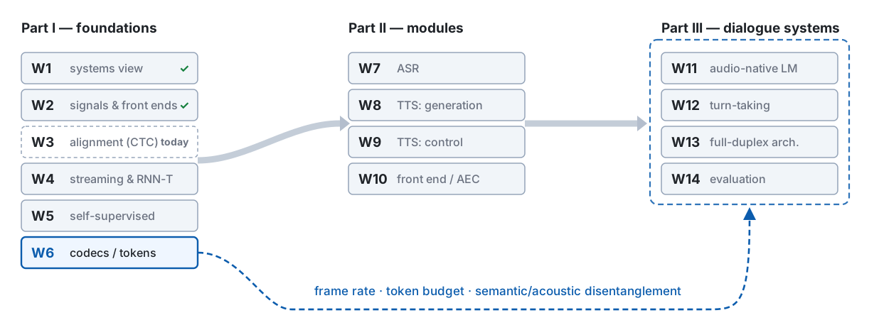
Last week, in one picture

Week 2 gave us the clock. Nobody gave us what each tick belongs to — and that gap is the whole of this week.

The same gap, in symbols — and on the three axes

Week 2 left us with 100 feature vectors per second, \mathbf{X} = (\mathbf{x}_1, \dots, \mathbf{x}_T). The training data gives each clip one line of text, \ell = (\ell_1, \dots, \ell_U) — and nothing in between.

Axis	This week’s question
Supervision	How do you train on (\mathbf{X}, \ell) when nobody says which frames belong to which symbol?
Representation	The label unit and the frame rate now constrain each other. Who gives way?
Latency	If every frame emits on its own, streaming is free — what did we pay for it?

Before Demo 1: what does speaking faster change?

Why	The last slide put the gap in symbols: T frames in, U symbols out, nothing in between. This demo shows that gap on a real voice, before any equation touches it.
What runs	A volunteer says 今天天氣很好 twice: at normal speed, then about twice as fast. Each take is trimmed of silence; the two spectrograms are drawn one above the other, aligned at the start, one column per 10 ms frame.
Watch for	The frame count T, the symbol count U, and anything on the screen that says which frames belong to which character. And: does T halve when the speed doubles?

Demo 1 — the same sentence, twice as fast

Demo 1. Before the plots appear: which numbers change between the two takes, and which stay the same?

The problem this week handles, in one picture

Speech recognition is sequence supervision under an unknown alignment. Every method this week is a way of handling that hidden variable.

Five things to leave with today

1. HMM forward and Viterbi are one recursion in two semirings — sum gives the probability of the sequence, max gives one best alignment, and they are not interchangeable.
2. CTC in full: the extended sequence \ell', the collapsing map \mathcal{B}, the recursion and its third term, the boundaries, P(\ell \mid \mathbf{X}) = \alpha_T(S) + \alpha_T(S-1), and the exact condition for zero probability, T < U + r.
3. The gradient is y^t_k - \gamma_t(k): a per-frame cross-entropy whose target is a soft alignment posterior. That one line explains the link to hybrid training and where peaky outputs come from.
4. Conditional independence — what the encoder sees versus what the outputs share are two different things.
5. CTC is an HMM with a special topology, and the three alignment families differ in inductive bias, not in kind.

Remedial: probability in four lines

Marginalisation: sum out what you cannot see

P(\ell \mid \mathbf{X}) \;=\; \sum_{\pi} P(\ell, \pi \mid \mathbf{X})

\pi is the thing we never observe — the alignment. If we cannot know it, we add up every value it could take.

Every equation today has this shape: a probability we want, written as a sum over a hidden alignment. The only question is how to do the sum without enumerating it.

• A hidden variable is not a nuisance to be guessed away; it is a dimension to be summed.
• The sum has exponentially many terms. Dynamic programming is what makes today possible.

Chain rule, then conditional independence

P(\pi \mid \mathbf{X}) \;=\; \prod_{t=1}^{T} P(\pi_t \mid \pi_{1:t-1}, \mathbf{X}) \;\;\xrightarrow{\;\text{assume}\;}\;\; \prod_{t=1}^{T} P(\pi_t \mid \mathbf{X}) \;=\; \prod_{t=1}^{T} y^t_{\pi_t}

The chain rule is exact. The arrow is an assumption: given \mathbf{X}, the symbol at frame t does not depend on the symbols at other frames.

This line is the whole assumption of CTC. Every pathology in the last hour of today — no output language model, homophones, peaky spikes — comes back to this arrow.

y^t_k is the network’s softmax output for symbol k at frame t. The network sees all of \mathbf{X}; the outputs see nothing of each other.

Log domain: products become sums, sums become log-sum-exp

\ln \prod_t y^t_{\pi_t} = \sum_t \ln y^t_{\pi_t}, \qquad \ln \sum_i e^{a_i} \;=\; a^{*} + \ln \sum_i e^{a_i - a^{*}}, \quad a^{*} = \max_i a_i

• A product of T probabilities shrinks like c^T. In float64 it can hit zero inside a single sentence.
• Subtracting a^{*} first keeps every exponent \leq 0: no overflow, and the largest term is computed exactly.
• Example. Two paths arrive at the same node with \ln p_1 = -1000, \ln p_2 = -1001; the node needs \ln(p_1 + p_2). Going back to probabilities fails: e^{-1000} = 0 in float64, so \ln(0 + 0) = -\infty. Factor out a^{*} = -1000 instead: -1000 + \ln(1 + e^{-1}) = -1000 + 0.313 = -999.687.

Two operations cover every algorithm today: (+, \times) in probability space is (\operatorname{logsumexp}, +) in log space, and (\max, \times) is (\max, +).

Notation for today

Symbol	Meaning
\mathbf{x}_t \in \mathbb{R}^d, \mathbf{X} = (\mathbf{x}_1, \dots, \mathbf{x}_T)	frame vectors from the W2 front-end; T frames
\ell = (\ell_1, \dots, \ell_U), U = \lvert \ell \rvert	the transcript, over vocabulary \mathcal{V}
\varnothing, \mathcal{V}' = \mathcal{V} \cup \{\varnothing\}	the blank, and the output alphabet with it
\ell', S = 2U + 1	\ell with a blank before, between and after every label
\pi \in \mathcal{V}'^{\,T}	a path: one output symbol per frame
\mathbf{u}^t, \mathbf{y}^t = \operatorname{softmax}(\mathbf{u}^t), y^t_k	logits, softmax, and one entry of it at frame t
\mathcal{L}_{\text{CTC}} = -\ln P(\ell \mid \mathbf{X}), \gamma_t(k)	the loss, and the alignment posterior P(\pi_t = k \mid \ell, \mathbf{X})
q_t \in \{1, \dots, N\}, \pi_i, a_{ij}, b_j(\mathbf{x}_t)	HMM side: state, initial, transition, emission
m	encoder lookahead in frames when streaming (W1 wrote it \ell; today \ell is the transcript)

The HMM in forty minutes

One model, three problems, one lattice

P(\mathbf{X} \mid W) \;=\; \sum_{q} \pi_{q_1}\, b_{q_1}(\mathbf{x}_1) \prod_{t=2}^{T} a_{q_{t-1} q_t}\, b_{q_t}(\mathbf{x}_t)

q = (q_1, \dots, q_T) is the hidden state sequence — it is the alignment. W fixes the topology: a chain of states per phone, left to right.

Rabiner’s problem	Question	Algorithm
Evaluation	How likely is \mathbf{X} under this W?	forward
Decoding	Which state sequence best explains \mathbf{X}?	Viterbi
Learning	Which a_{ij}, b_j make the data most likely?	Baum–Welch (forward–backward)

Forward: add every way of arriving

\alpha_t(j) = b_j(\mathbf{x}_t) \sum_{i} \alpha_{t-1}(i)\, a_{ij}, \qquad \alpha_1(j) = \pi_j\, b_j(\mathbf{x}_1), \qquad P(\mathbf{X} \mid W) = \sum_j \alpha_T(j)

Viterbi is forward with the sum replaced by max

\delta_t(j) = b_j(\mathbf{x}_t)\, \max_{i}\, \delta_{t-1}(i)\, a_{ij}, \qquad \text{then backtrack the argmax.}

Space	“add every way”	“keep the best way”	Gives
probability	(+, \times)	(\max, \times)	forward / Viterbi
log	(\operatorname{logsumexp}, +)	(\max, +)	what the code actually runs

Same lattice, same recursion, different semiring. This week: HMM and CTC. W4: the RNN-T lattice. W7: prefix beam search. You will see this table three more times.

Misconception 1 — “forward gives the probability of the best alignment”

Forward is a sum over every alignment, \sum_q P(\mathbf{X}, q \mid W) — how likely is the audio under the words. Viterbi is a max, \max_q P(\mathbf{X}, q \mid W) — how likely is the audio under the single best state sequence.

The best single alignment usually carries a small fraction of the total. And the argmax over paths need not agree with the argmax over label sequences — many weak paths can outvote one strong one.

Why triphones, and why tying

Week 2’s fact: articulators cannot jump, so a phone sounds different depending on its neighbours.

The HMM’s answer: write the neighbours into the unit. A triphone /s-k+i/ is its own model, distinct from /u-k+o/.

• The count explodes: with \sim 40 phones, 40^3 = 64{,}000 triphones, each with several states — most never seen in training.
• Tying shares parameters across states that behave alike. A decision tree asks phonetic questions (“is the left neighbour a nasal?”) and groups the leaves.

The unit absorbs the context because the model cannot: an HMM state sees one frame, and the outputs are conditionally independent given the state. Remember that sentence — it returns for CTC.

The hybrid recipe, and the bootstrap it needs

You need a working recogniser before you can train the recogniser. The targets are hard — one state per frame — and they are only as good as the model that produced them.

Misconception 2 — “HMMs are obsolete, skip them”

• W4 — the RNN-T lattice is a two-dimensional version of today’s grid, and its forward is the same recursion.
• W7 — prefix beam search for CTC is forward over label prefixes instead of paths.
• W13 — the finite-state route to full duplex is a decoding problem on a state machine: which state is the conversation in, given the audio so far?
• W10 / W12 — a semantic endpoint decision is a Viterbi-style question with a latency constraint.

The HMM is not a system you will deploy. It is the grammar of every alignment algorithm you will read for the rest of this course.

CTC: marginalise the alignment

The trick: one extra symbol, and a collapsing map

\mathcal{B} maps a path of length T to a label sequence: merge adjacent repeats, then delete every \varnothing.

Before Demo 2: list the paths, check the sum

Why	P(\ell \mid \mathbf{X}) is a sum over every path that \mathcal{B} collapses to \ell. Before deriving a recursion for that sum, look at what it sums over; once the recursion is derived, check it against the brute-force sum.
What runs	One terminal program, pure numpy, used twice. Next slide: list the paths for “aa” and “aba” on paper, then let the program list them. After the forward recursion: a random \mathbf{y}^t, every path’s probability summed, next to the forward table filled column by column — then T = 500.
Expect	The two sums agree to floating-point error; if they do not, the recursion is wrong. Watch how fast the number of paths grows with T, whether every pair (\ell, T) has a path at all, and what the linear-domain table does at T = 500.

Paths: write them out before the program does

Demo 2, first half — on paper first. Vocabulary \{a, b\} plus \varnothing. Write every path of length T = 3 that collapses to “aa”, and every one that collapses to “aba”. Then T = 4 for “aa”.

\ell	T	paths in \mathcal{B}^{-1}(\ell)	count
aa	2	—	0
aa	3	\mathsf{a}\varnothing\mathsf{a}	1
aba	3	\mathsf{aba}	1
aa	4	\mathsf{aa}\varnothing\mathsf{a} · \mathsf{a}\varnothing\mathsf{aa} · \mathsf{a}\varnothing\mathsf{a}\varnothing · \mathsf{a}\varnothing\varnothing\mathsf{a} · \varnothing\mathsf{a}\varnothing\mathsf{a}	5
ab	4	\mathsf{aaab} · \mathsf{aabb} · \mathsf{aab}\varnothing · … · \varnothing\varnothing\mathsf{ab}	15 of 3^4 = 81 candidates

Two equations that are the same equation

	HMM	CTC
what is modelled	P(\mathbf{X} \mid W) — generative	P(\ell \mid \mathbf{X}) — discriminative
the hidden alignment	state sequence q	path \pi
the sum	\displaystyle\sum_{q} \pi_{q_1} b_{q_1}(\mathbf{x}_1) \prod_{t=2}^{T} a_{q_{t-1}q_t} b_{q_t}(\mathbf{x}_t)	\displaystyle\sum_{\pi \in \mathcal{B}^{-1}(\ell)} \prod_{t=1}^{T} y^t_{\pi_t}
per-frame factor	transition \times emission	softmax output, nothing else

Both are a sum over alignments of a product over frames. CTC has no transition term and a discriminative emission. Everything else — the lattice, the recursion, the semiring — carries over.

The extended sequence \ell': where a path is allowed to go

\ell' = (\varnothing, \ell_1, \varnothing, \ell_2, \dots, \ell_U, \varnothing), length S = 2U + 1. A path is a walk on this graph, one node per frame.

Forward on the CTC lattice

\alpha_t(s) = y^t_{\ell'_s}\Bigl(\alpha_{t-1}(s) + \alpha_{t-1}(s-1) + [\ell'_s \neq \varnothing \,\wedge\, \ell'_s \neq \ell'_{s-2}]\;\alpha_{t-1}(s-2)\Bigr)

Boundaries, the end, and what the table cost

Quantity	Value	Why
\alpha_1(1)	y^1_{\varnothing}	the path may open with a blank
\alpha_1(2)	y^1_{\ell_1}	or with the first label
\alpha_1(s),\; s > 2	0	unreachable in one frame
\alpha_t(s),\; s < S - 2(T-t) - 1	0	cannot reach the end in the frames left
P(\ell \mid \mathbf{X})	\alpha_T(S) + \alpha_T(S-1)	the last frame is a blank, or the last label

Exponentially many paths, O(TS) cells. The same idea as the HMM forward, O(TN^2) — here every cell has at most three predecessors, so the N^2 becomes 3S.

Misconception 3 — “you need T \geq 2U + 1 frames”

T < U + r \;\Rightarrow\; \mathcal{B}^{-1}(\ell) = \varnothing \;\Rightarrow\; P(\ell \mid \mathbf{X}) = 0 \;\Rightarrow\; \mathcal{L}_{\text{CTC}} = \infty, \qquad r = \bigl|\{u : \ell_u = \ell_{u+1}\}\bigr|

Where the inf comes from in practice

Who eats the frames: a 10 ms hop gives 100 per second; a 4\times subsampling encoder leaves 25. A fast talker with character-level labels can push U + r past that.

Who inflates U: character-level Mandarin (one symbol per character), letter-level English, any label unit finer than the encoder’s clock can afford.

zero_infinity=True replaces an infinite loss by zero and a gradient by nothing. It hides the utterance; it does not fix it. Count U + r against T first.

When the loss is inf	Check, in this order
1	U + r against T — the label is too long for the frames
2	a label symbol that is not in \mathcal{V} (mapped to blank or to an unknown id)
3	only then, numerics: are you summing in the log domain?

Check the recursion against brute force

With every y^t_k = 1/3 (vocabulary \{a, b, \varnothing\}), each path has probability 3^{-T}, so P(\ell \mid \mathbf{X}) must equal \lvert \mathcal{B}^{-1}(\ell) \rvert \cdot 3^{-T} — a number you can check by hand.

\ell	T	brute force	forward table	match
aa	2	0 / 9	0	✓
aa	3	1 / 27	0.037037	✓
aba	3	1 / 27	0.037037	✓
aa	4	5 / 81	0.061728	✓
ab	4	15 / 81	0.185185	✓

Demo 2, live version. Same script, random \mathbf{y}^t: enumeration and forward agree to floating-point error. Then T = 500 with \lvert \mathcal{V}' \rvert = 32.

From the loss to its gradient: paths through one cell

The forward table gives one number, P = P(\ell \mid \mathbf{X}). Training needs \partial \mathcal{L}_{\text{CTC}} / \partial u^t_k at every (t, k).

P = \sum_{\pi \in \mathcal{B}^{-1}(\ell)} \prod_{t'=1}^{T} y^{t'}_{\pi_{t'}} \quad\Longrightarrow\quad \frac{\partial P}{\partial y^t_k} = \frac{1}{y^t_k} \sum_{\pi \in \mathcal{B}^{-1}(\ell),\; \pi_t = k} P(\pi \mid \mathbf{X})

Paths through a cell: ways in \times ways out. The ways in, \alpha_t(s), are already in the forward table; the ways out need a second table, filled from the end.

Backward: the same recursion, run from the end

\beta_t(s) = \beta_{t+1}(s)\, y^{t+1}_{\ell'_s} + \beta_{t+1}(s+1)\, y^{t+1}_{\ell'_{s+1}} + [\,\cdot\,]\; \beta_{t+1}(s+2)\, y^{t+1}_{\ell'_{s+2}}, \qquad \beta_T(S) = \beta_T(S-1) = 1

The gradient: soft targets, per frame

\gamma_t(k) \;=\; \frac{1}{P(\ell \mid \mathbf{X})} \sum_{s:\, \ell'_s = k} \alpha_t(s)\, \beta_t(s) \;=\; P(\pi_t = k \mid \ell, \mathbf{X})

\frac{\partial \mathcal{L}_{\text{CTC}}}{\partial u^t_k} \;=\; y^t_k - \gamma_t(k)

Cross-entropy’s y_k - e_k, with the one-hot \mathbf{e} replaced by the posterior \gamma_t(\cdot).

Where y^t_k - \gamma_t(k) comes from: three lines

1. \mathcal{L}_{\text{CTC}} = -\ln P with P = P(\ell \mid \mathbf{X}), and P = \sum_s \alpha_t(s)\,\beta_t(s) holds for this t (the backward slide).

2. Inside \alpha_t(s) only the factor y^t_{\ell'_s} involves \mathbf{y}^t; \beta_t(s) does not (that is what the convention bought). So \frac{\partial P}{\partial y^t_k} = \frac{1}{y^t_k}\sum_{s:\, \ell'_s = k} \alpha_t(s)\,\beta_t(s) \qquad\Rightarrow\qquad \frac{\partial \mathcal{L}}{\partial y^t_k} = -\frac{\gamma_t(k)}{y^t_k}

3. Softmax Jacobian \dfrac{\partial y^t_j}{\partial u^t_k} = y^t_j\,(\delta_{jk} - y^t_k), then chain rule over j: \frac{\partial \mathcal{L}}{\partial u^t_k} = \sum_j \Bigl(-\frac{\gamma_t(j)}{y^t_j}\Bigr)\, y^t_j\,(\delta_{jk} - y^t_k) = -\gamma_t(k) + y^t_k \underbrace{\sum_j \gamma_t(j)}_{=\,1} = y^t_k - \gamma_t(k)

Read it as a cross-entropy

	Hybrid DNN–HMM (step 3 of the recipe)	CTC
loss per frame	cross-entropy	cross-entropy
gradient on logits	y^t_k - e_k	y^t_k - \gamma_t(k)
the target	hard: one state, from a forced alignment	soft: a posterior over symbols
who made the target	the previous model, once	the current model, every step
needs a bootstrap	yes	no

CTC is per-frame cross-entropy against a soft alignment recomputed at every update. That is the whole difference from hybrid training — and it is also where the pathologies begin.

Numbers underflow before you notice

y^{T} < 5 \times 10^{-324} \iff T > \frac{-323.3}{\log_{10} y}, \qquad y = 0.1:\; T > 323.3, \text{ so the product is } 0 \text{ from } T = 324

One \beta, two conventions — read the paper you cite

	Graves et al., ICML 2006	Graves, Supervised Sequence Labelling, 2012 (this deck)
\beta_t(s) runs over frames	t, \dots, T — includes y^t	t+1, \dots, T — excludes y^t
P(\ell \mid \mathbf{X}) at frame t	\sum_s \alpha_t(s)\beta_t(s) / y^t_{\ell'_s}	\sum_s \alpha_t(s)\beta_t(s)
gradient on the logits	carries an extra 1/y^t_k inside the sum	y^t_k - \gamma_t(k)

Neither is wrong; mixing them is. A \beta that starts at t plus the book’s gradient raises no error — it just trains slowly and strangely.

When CTC goes wrong

Before Demo 3: a trained CTC model, one sentence

Why	Every posterior so far was made up: uniform, random, or drawn. Now a real character-level CTC model on one LibriSpeech sentence, with two questions: what does the blank do in real speech, and what happens to the loss when the text is too long for the audio?
What runs	wav2vec2-base-960h on the CPU. First a heat-map: one column per 20 ms frame, one row per symbol, the blank row enlarged at the bottom, non-speech frames shaded grey. Later, ctc_loss on the same logits, with the text lengthened one character at a time past U + r = T.
Watch for	The blank row where there is no grey: if blank meant silence, it would be low there. For the loss, the zero-probability condition already says where it breaks; watch what the loss looks like there, and what zero_infinity turns it into.

Demo 3 — a blank heat-map

Demo 3. Before the plot: in a sentence with no pauses, what fraction of frames will the blank win? Write down a number.

Measured on the sentence	value
frames T (after the model’s own subsampling)	292 (5.86 s, one frame per 20 ms)
characters U, repeats r, U + r	89 (73 letters + 16 |), 2, 91
frames where \varnothing is the argmax	149 / 292 = 51 %
frames inside speech where \varnothing is the argmax	94 / 232 = 41 %

Misconception 4 — “the blank is silence”

The blank is the symbol for “no new label at this frame.” It is bookkeeping, not acoustics.

• Inside a vowel that lasts 100 ms, one frame emits the label and the other nine emit \varnothing. They are not silent.
• A silent frame can also be \varnothing — but so can nearly every voiced one. Silence is a sufficient reason for blank, never a necessary one.

If you ever find yourself “explaining” a blank-dominated posterior by pauses, look at Demo 3’s last row again: blank wins 4 frames in 10 inside speech. W1’s \varnothing — “say nothing this frame” — is the same kind of object.

Peaky: one spike per label, blanks everywhere else

Peaky, measured: one word

Six letters on eight frames, blanks in the gaps, the word boundary | emitted like any other symbol. This is what Demo 3’s heat-map looks like up close — and why “4 in 10” inside speech is not a majority: every label still needs at least one frame.

Why peaky: the target chases the model

From the gradient y^t_k - \gamma_t(k), with \gamma recomputed from the current model at every step:

Zeyer, Schlüter & Ney (2021) give a formal analysis of this as a convergence property of the CTC loss under gradient descent; on a toy example they prove a feed-forward network from uniform initialisation converges to peaky behaviour, and show a related loss with a label prior does not.

Misconception 5 — “CTC’s argmax gives you the boundaries”

Phone level: no. The spike is where the model chose to emit, not where the sound starts or ends. A peaky output puts the spike somewhere inside the segment, and nothing in the loss says where. For phone boundaries use a hybrid forced alignment or a dedicated aligner.

Word level: yes, routinely. A CTC forced alignment — Viterbi through \ell' with the known transcript — gives word timestamps good enough for subtitles and for training data:

• MMS ships a CTC forced aligner (the backbone of the torchaudio alignment tutorial)
• WhisperX aligns Whisper’s output with a wav2vec 2.0 CTC model to get word-level times

“CTC cannot align” overshoots as badly as “CTC alignments are ground truth.” The right statement is about granularity.

Forcing too much text: inf, and what zero_infinity hides

Demo 3, second half. Same logits, correct transcript → a finite loss. Now append text until U + r > T.

	loss	gradient	what you learn
correct transcript	finite	y^t_k - \gamma_t(k)	the sentence trains normally
too long, zero_infinity=False	inf	nan	the batch is poisoned — you notice
too long, zero_infinity=True	0	0	the sentence silently contributes nothing

Row three is the dangerous one. A data pipeline that trims audio but not text, or an encoder with one stride too many, produces a training set that looks fine and trains on a fraction of itself.

Conditional independence, as a graph

Every arrow from \mathbf{X} is there; every arrow between outputs is missing. The assumption lives only in the top row.

Conditional independence: what the encoder sees, what the outputs share

Statement	Verdict
“The encoder sees the whole utterance”	true — \mathbf{y}^t is computed from all of \mathbf{X}, or \mathbf{x}_{1:t+m} when streaming with m frames of lookahead
“The outputs are conditionally independent”	true — P(\pi \mid \mathbf{X}) = \prod_t y^t_{\pi_t}: no output is conditioned on another
“CTC has no language model at all”	overshoots — acoustic context carries linguistic information, and the encoder uses it
“CTC needs no language model”	overshoots — nothing at the output couples one symbol to the next; fusion gains are large

The assumption is about the output layer, not about the network. Whatever the acoustics can support, the encoder can learn; whatever needs the previous symbol, it cannot.

Misconception 6 — “CTC needs no LM” / “CTC has no LM”

Both overshoot; the previous slide has the precise version. Here is why it matters more for this room:

• In Mandarin, the acoustic form of a syllable underdetermines the character far more often than in English: homophones are dense, and a tone error is a different character, not a mispronunciation.
• With outputs conditionally independent, a greedy CTC decode picks each character on acoustics alone. The context that would disambiguate is textual — exactly what the output layer cannot see.

My judgement, not consensus: the conditional-independence cost bites harder in Mandarin than in English, so the gain from an external LM should be larger. W7 will test this with numbers.

The vocabulary is decided before the loss

CTC needs a fixed, finite \mathcal{V}. Everything downstream follows from that choice:

Choice of \mathcal{V}	U for one second of speech	Subsampling you can afford
characters	large	little
phones	medium	some
BPE / word pieces	small	more

Taiwanese has no single orthography — Hàn-jī, Tâi-lô and Pe̍h-ōe-jī coexist. “Which symbols are in \mathcal{V}” must be decided before the first line of training code, and it fixes U, hence the floor on T, hence the encoder’s stride.

W1’s orthography gap for local languages has its first engineering consequence here: the label set is a modelling decision that precedes the loss, not a preprocessing detail.

CTC is an HMM

CTC as an HMM with a special topology

	HMM (GMM or hybrid)	CTC
states	phone states, N of them, tied	the S = 2U + 1 positions of \ell'
allowed transitions	as the topology says, with a_{ij}	stay · +1 · +2 under the condition, all with weight 1
emission	generative b_j(\mathbf{x}_t), or scaled posterior	discriminative y^t_k, shared across positions with the same symbol
training	Viterbi (hybrid) or full-sum (Baum–Welch)	full-sum (forward), always
alignment	hard (hybrid) or soft (full-sum)	soft, every step
direction	P(\mathbf{X} \mid W)	P(\ell \mid \mathbf{X})

Zeyer, Beck, Schlüter & Ney (2017) formulate generalised full-sum hybrid HMM training and identify CTC as a special case. Raissi et al. (SLT 2022) compare the two under one from-scratch full-sum setup.

Misconception 7 — “CTC is a loss, an HMM is a model; you cannot compare them”

The previous table is the comparison. Put the two sums side by side once more:

\sum_{q} \pi_{q_1} b_{q_1}(\mathbf{x}_1) \prod_{t=2}^{T} a_{q_{t-1}q_t}\, b_{q_t}(\mathbf{x}_t) \qquad\text{vs.}\qquad \sum_{\pi \in \mathcal{B}^{-1}(\ell)} \prod_{t=1}^{T} y^t_{\pi_t}

Drop the transition probabilities, replace the generative emission by a softmax, fix the topology to \ell', and train full-sum: the left sum becomes the right one. A loss that sums over alignments is a model of alignments.

• What CTC removed: the bootstrap, and the duration model.
• What it kept: the lattice, the recursion, the semiring, the forward–backward gradient.

Three families of alignment, three inductive biases

	frame-level (hybrid)	CTC	attention (W4)
alignment	hard, contiguous	monotonic, many-to-one, blank-padded	soft, learned, need not be monotonic
duration model	yes (a_{ij})	none	none, but no blank either
streaming	yes	yes, encoder permitting	not without extra machinery

Misconception 8 — “blank means the same thing in every loss”

	CTC (today)	RNN-T (W4)
what \varnothing means	this frame emits no new label	consume one frame; advance time
labels per frame	exactly one symbol from \mathcal{V}'	zero, one, or several labels, then a blank
the lattice	T \times S, one axis is \ell'	T \times (U+1), two independent axes
output dependency	none	yes — a prediction network sees the previous labels

Same word, same glyph, different semantics. Next week the blank stops meaning “nothing” and starts meaning “next frame, please” — and that change is what buys back the output dependency CTC gave up.

Back to the three axes

Representation: T \geq U + r is a floor on the frame rate

W2 asked who decides the frame rate and answered “the hop, times every stride.” Today adds the other side: the label unit sets how slow the clock is allowed to get. Stride and vocabulary are one decision.

Latency and supervision: what CTC buys, what it costs

Axis	What CTC does	The price
Latency	every frame emits on its own, so a causal encoder streams with no extra decoder state; algorithmic latency is W1’s D_{\text{alg}} of the encoder alone — no decoder adds to it	no output dependency — the symbol you just emitted cannot inform the next
Supervision	(\mathbf{X}, \ell) pairs are enough; the alignment is summed out and never annotated	no duration model; the target chases the model (peaky); the vocabulary must be fixed first

CTC made streaming and alignment-free training almost free. W4 pays for the output dependency (RNN-T); W7 pays for the language model (fusion). Nothing today was free — it was deferred.

What this week put on the three axes

Axis	What we now know
Supervision	Audio plus a transcript is enough: the alignment is summed out. The gradient is a per-frame cross-entropy against a soft alignment, recomputed every step.
Representation	T \geq U + r: label unit and encoder stride are one decision, and the vocabulary is fixed before the loss exists.
Latency	Per-frame emission makes CTC streamable for the encoder’s lookahead alone. The output dependency it gives up returns next week.

Every alignment method handles one hidden variable. HMM and CTC sum it out on the same lattice; they differ in what each refuses to model.

Reading, and next week

Read this week

• Graves, Supervised Sequence Labelling with Recurrent Neural Networks, Springer 2012, Ch 7 — the derivation you saw, in the notation you saw
• Jurafsky & Martin, Speech and Language Processing, 3rd ed. draft, App A (HMMs) and the CTC section of Ch 16

If one thing today was new to you, make it this one

• Hannun, Sequence Modeling with CTC, Distill 2017 — an interactive walkthrough of the path set and the collapsing map. Editorially reviewed, not a peer-reviewed paper; read it for the pictures

Next week — sequence models and streaming architectures

The blank changes meaning, the lattice gains a second axis, and the encoder learns to look ahead by exactly as much as the latency budget allows: Transformer, Conformer, RNN-T.