Speech Signals, Auditory Front-Ends, and the Physics of Representation

Speech Processing & Human–Machine Interaction · Week 2

Hung-Shin Lee

From air to numbers

Where we are: week 2 of 14

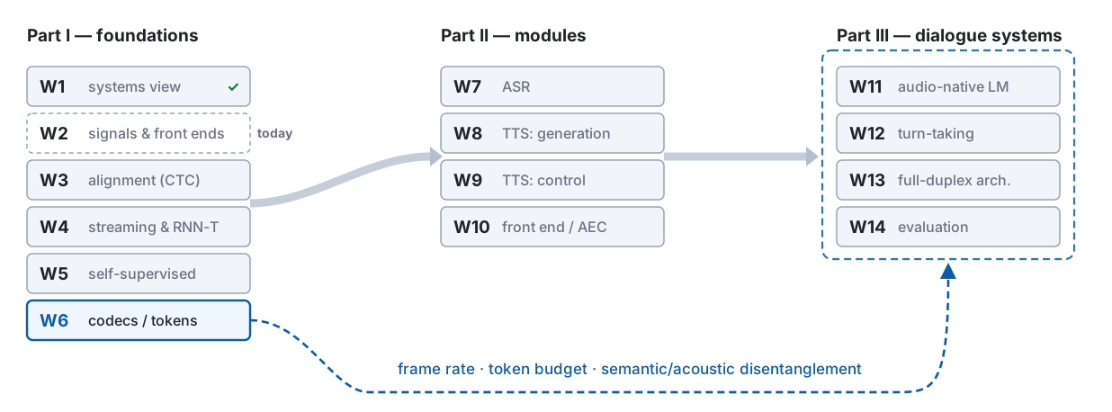
Last week, in one picture

Week 1 priced every delay in frames. Nobody said how long a frame is, or who decides — that is the first question today answers.

The problem this week handles, in one picture

The front end decides what every later layer is allowed to know — and how long it waits to know it. Today is the semester’s only systematic pass through that pipeline.

Sampling: a waveform becomes a list of numbers

x(n) = x_c(nT_s), \qquad f_s = 1/T_s

A sampled signal can represent frequencies only up to f_s/2 — the Nyquist frequency.

16 kHz sampling means 8 kHz of bandwidth. They are two different numbers, and they get mixed up constantly.

• 8 kHz sampling → 4 kHz bandwidth: the telephone
• 16 kHz sampling → 8 kHz bandwidth: what most ASR models were trained on
• 24 or 48 kHz sampling: what TTS and audio-quality evaluation need

Energy above f_s/2 does not disappear. It folds back.

A 7 kHz tone sampled at 8 kHz produces exactly the same samples as a 1 kHz tone — one line says why: at the sample instants n, \cos\!\bigl(2\pi \tfrac{f}{f_s} n\bigr) = \cos\!\bigl(2\pi n - 2\pi \tfrac{f}{f_s} n\bigr) = \cos\!\bigl(2\pi \tfrac{f_s - f}{f_s} n\bigr). Nothing downstream can tell them apart.

So before lowering the sample rate, low-pass first. A good resampler does this for you; dropping every other sample does not.

Misconception — “a higher sample rate is always better”

The right sample rate depends on the task. The wrong one is whichever differs from what the model was trained on.

What you did	What happens
Fed 44.1 kHz audio to a 16 kHz model without resampling	No error. Everything sounds slowed down to the model; accuracy collapses
Upsampled 8 kHz telephone speech to 16 kHz and called it wideband	No error. The top half of the spectrum is empty; the model has never seen that
Downsampled by dropping samples	No error. Aliasing, as on the last slide

None of these raises an exception. Sample-rate mismatch is the most common silent bug in a speech project.

How speech is made

A tube and a buzzer

The vocal tract is a tube whose shape you can change, driven by a periodic source — the vocal folds.

• The buzzer sets how fast the pulses come: the fundamental frequency, F_0
• The tube decides which frequencies get through: its resonances are the formants
• Move your tongue and lips, and you reshape the tube. The buzzer does not care

We will stretch this picture all semester: a vocoder models the two parts separately (W8); voice cloning has to copy both (W9).

Every metaphor breaks somewhere. Keep a list of where this one does — we collect it in ten minutes.

The source–filter model in one line

s(n) = e(n) * h(n) \quad\Longleftrightarrow\quad S(\omega) = E(\omega)\,H(\omega)

Convolution in time is multiplication in frequency. We use this fact four times this semester; this is the first.

Before Demo 1: a spectrogram you can talk into

Why	The source–filter model puts the vowel in the filter — the formants — and the pitch in the source, F_0. This demo shows both live from a microphone, so you can move one and watch which numbers follow.
What runs	A microphone into a 4 s scrolling spectrogram (5 ms or 30 ms window), an autocorrelation F_0 track, and an LPC (F_1, F_2) dot on a vowel chart; all the signal processing is plain numpy and scipy. Used three times today: vowels now, then the same sound under two window lengths, then Mandarin tones.
Watch for	Now: where the dot goes for /a/, /i/, /u/, and the path it takes from /i/ to /a/. Later: what the window length changes on the same sound, and whether a tone keeps its shape when the sentence becomes a question.

Two formants are enough to tell vowels apart

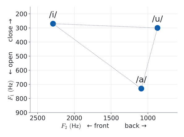
Vowels live in a two-dimensional space:

• F_1 tracks how open the mouth is
• F_2 tracks how far forward the tongue is

/i/, /a/, /u/ sit at the corners. Every other vowel is somewhere inside.

Demo 1. Say /a/ … /i/ … /u/. Then slide slowly from /i/ to /a/ and watch the dot.

The minimum phonetics you need for the next three weeks

Term	What it means	Where it comes back
phone	an acoustic event — what was physically produced	W5: what SSL units partly capture
phoneme	a contrastive unit inside one language — what distinguishes words	W3: what the HMM states model
consonants	three dimensions: place, manner, voicing	W3: decision-tree questions
vowels	two dimensions: height and backness → F_1, F_2	today

One phoneme, several phones: the /t/ in top, stop and butter are physically different sounds that English treats as the same unit.

A phone is physics. A phoneme is a decision made by a language. Confusing the two is why “discrete unit = phoneme” sounds plausible — and is wrong (W5).

Coarticulation: one fact, two weeks of the course

Articulators cannot jump. The gesture for each sound overlaps with its neighbours, so the same phone sounds different depending on what is next to it.

The /k/ in key and the /k/ in coo are made in different places — your tongue is already preparing the vowel.

Week	What it does with this fact
W3 HMM	writes the context into the unit itself: the triphone — /k/ between /s/ and /i/ is its own model
W5 SSL	hides a stretch of audio and asks the model to predict it from the context — which works only because the context carries information about it

The same physical fact is a nuisance for one generation of systems and the training signal for the next.

Anatomy of a stop: the shortest events in speech

• closure — the tract is shut; near silence, tens of milliseconds or more
• burst — the release; a few milliseconds
• VOT — from release until voicing starts; this is what separates ㄅ from ㄆ

Look at the blue bar. One standard analysis window is longer than the burst and comparable to the VOT. Hold that thought.

Where the tube-and-buzzer picture breaks

1. Fricatives and bursts have no periodic source. /s/ is turbulence, not buzzing. Whisper has no F_0 at all
2. The length of the tube belongs to the speaker. A shorter vocal tract scales every formant up. So the filter carries who, not only what
3. In a tone language, the source carries words. Mandarin mā / má / mǎ / mà differ only in F_0

“The source is who is speaking, the filter is what they say” is a simplification that quietly assumes English. For Mandarin, Taiwanese and Hakka it is wrong in both directions.

Points 2 and 3 matter more than point 1, and they come back in W6, W9 and W12.

LPC: the source–filter model you can actually compute

Model the tube as an all-pole filter, and predict each sample from the previous p:

H(z) = \frac{1}{1 - \sum_{i=1}^{p} a_i z^{-i}} \qquad\qquad \hat{s}(n) = \sum_{i=1}^{p} a_i\, s(n-i)

• The coefficients a_i describe the envelope — the filter
• Whatever cannot be predicted, s(n) - \hat{s}(n), is the excitation — the source
• The red dot in Demo 1 came from exactly this: solve for a_i, find the poles, read off the formants

It is the core of classical speech codecs (CELP, and the speech mode of Opus), and the starting point of LPCNet (W8).

Seeing speech

A spectrum is a set of inner products

Euler: \; e^{j\theta} = \cos\theta + j\sin\theta. A complex exponential is a cosine and a sine carried in one number.

The DFT asks, for each frequency k: how much of this pattern is in my signal?

X(k) = \langle \mathbf{x}, \mathbf{b}_k \rangle = \sum_{n=0}^{N-1} x(n)\, e^{-j2\pi kn/N}, \qquad \mathbf{b}_k(n) = e^{j2\pi kn/N}

The patterns are orthogonal, \langle \mathbf{b}_k, \mathbf{b}_l \rangle = N\delta_{kl}, so the X(k) are coordinates in a new basis. Nothing is lost.

• |X(k)| — the magnitude: how long the projection is
• \angle X(k) — the phase: how far that pattern must be shifted to line up with the signal

To analyse a moving signal, cut it into pieces

Speech changes every few tens of milliseconds, so one spectrum of the whole utterance is useless. Take short, overlapping pieces, and a spectrum of each:

X(m,k) = \sum_{n} x(n)\, w(n - mH)\, e^{-j2\pi kn/N}

Symbol	Name	What it is
L	window length	how many samples w covers — 25 ms is typical for ASR
H	hop	how far the window moves each step — 10 ms is typical
N	FFT size	how many frequency points we compute, N \geq L

Three knobs. They control three different things, and most confusion about spectrograms comes from mixing them up.

The window sets the frequency resolution

Cutting out a piece is multiplying by a window. Multiplication in time is convolution in frequency — our theorem again, the other way round. Every spectral line gets smeared into the shape below.

• Main-lobe width \approx 2f_s/L (rectangular) or 4f_s/L (Hann): longer window, finer resolution
• Hann pays a main lobe twice as wide to push the side lobes from -13 dB down to -31 dB

Where 2f_s/L comes from

A rectangular window of L samples is L ones in a row. Its spectrum is a geometric sum:

W(f) = \sum_{n=0}^{L-1} e^{-j2\pi f n/f_s} \quad\Longrightarrow\quad |W(f)| = \left|\frac{\sin(\pi f L/f_s)}{\sin(\pi f/f_s)}\right|, \qquad \text{zero whenever } \tfrac{fL}{f_s} \in \{\pm 1, \pm 2, \dots\}

First zero at f_s/L, so the main lobe is 2f_s/L wide. Centre the window at n = 0 and Hann is w(n) = \tfrac12 + \tfrac12\cos(2\pi n/L): the cosine is two complex exponentials, so its spectrum is three copies of W with weights \tfrac12, \tfrac14, \tfrac14, shifted by 0 and \pm f_s/L.

Same sound, two window lengths

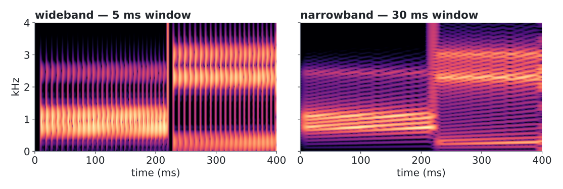
	Wideband — 5 ms	Narrowband — 30 ms
Main lobe (Hann)	800 Hz	133 Hz
You can see	glottal pulses as vertical stripes; formants as broad bands	individual harmonics as horizontal lines

Demo 1, again. I freeze the display, then switch the window. It is the same two seconds of sound.

What a 25 ms window cannot see

ASR’s standard window sits toward the narrowband side, and it gives up something at both ends.

Too slow for	Too coarse for
the burst of a stop — a few ms	two adjacent harmonics of a low voice — only just: 160 Hz main lobe vs. F_0 \approx 100 Hz
VOT — the cue separating ㄅ from ㄆ	two speakers whose F_0 are close

Remember the blue bar under the stop? That was this window.

25 ms is not the right answer. It is a compromise that happens to suit recognising words — and it quietly decides what every later layer is allowed to know.

Misconception — “a bigger n_fft gives better resolution”

Two tones 60 Hz apart. Left → middle: N = 400 \to 4096 — smoother, still one bump. Middle → right: L = 25 \to 50 ms — two peaks.

Zero-padding samples the same smeared spectrum more densely. Only a longer window un-smears it.

Hop sets the clock. The window sets the lookahead.

• The hop H is the frame shift — \Delta = H / f_s in seconds. Frame rate = f_s / H. This is last week’s \Delta
• A frame stamped at time t needs samples up to t + L/2. That is lookahead, paid before any model runs

Knob	Decides
window L	frequency resolution and lookahead
hop H	frame rate — the clock every later layer ticks on
FFT size N	spacing of the frequency points. Nothing else

Who decides the frame rate? The hop, times every stride after it

\text{frame rate} = \frac{f_s}{H \cdot \prod_i s_i}

Every stride s_i slows the clock, and nothing downstream can run faster than the clock it is given. That is the first answer to who decides the frame rate.

Why take the log

\log|S| = \log|E| + \log|H|

1. Dynamic range. Speech energy spans several orders of magnitude; perceived loudness is closer to logarithmic than linear
2. Products become sums. A microphone or a room multiplies the spectrum by some response C(\omega). After the log, that is a constant vector added to every frame

Subtract each dimension’s mean over the utterance, and most of the channel is gone. That is why mean normalisation (CMVN) works at all — it would be meaningless on a linear scale.

A product has turned into a sum again — and it will not be the last time today.

The ear is a filterbank, and mel is its engineering sketch

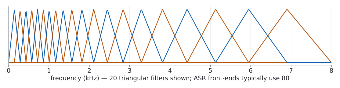
The cochlea analyses sound with filters that get wider as frequency goes up. Mel imitates that: narrow triangles at the bottom, wide ones at the top.

m = 2595 \log_{10}\!\left(1 + \frac{f}{700}\right) \qquad\qquad \mathbf{y}_m = \log\!\left(\mathbf{M}\,|\mathbf{X}_m|^2 + \epsilon\right)

• \mathbf{M} is a fixed matrix, about 80 \times 257: 257 frequency points in, 80 numbers out
• The mel scale is a psychoacoustic approximation, fitted to listening experiments. It is not physics

Masking: what the ear cannot hear, codecs do not send

A strong component raises the hearing threshold around it: a weaker one nearby can be present and inaudible.

• MP3, AAC, Opus spend no bits on what is masked — a psychoacoustic model written by hand
• Neural codecs (W6) have no such model; their losses push them there indirectly

Misconception — “MFCC carries more information than log-mel”

MFCC is log-mel, plus one more linear step that throws things away:

\text{log-mel (80 dims)} \;\xrightarrow{\;\text{DCT}\;}\; \text{keep the first 13 coefficients} \;=\; \text{MFCC}

• The DCT decorrelates the dimensions. Truncating it keeps the smooth spectral envelope and drops the fine detail
• That was exactly right for GMMs with diagonal covariance, which assume uncorrelated dimensions
• A neural network does not need decorrelated inputs, and can use the detail MFCC discarded

MFCC did not lose to log-mel because it was worse. The classifier changed, and the reason for the last step disappeared.

Misconception — “a spectrogram is just an image”

It looks like one, and image models do work on it — up to a point.

	Natural image	Spectrogram
Shift a pattern horizontally	same object, elsewhere	same sound, later — fine
Shift a pattern vertically	same object, elsewhere	a different vowel, or a different speaker
The two axes	same kind of quantity	time and frequency — not interchangeable
Two objects overlap	one hides the other	they add; both are still there

Translation invariance holds along time and fails along frequency. An architecture that treats both axes alike is assuming something false.

What the spectrogram throws away

Before Demo 2: what does the spectrogram throw away?

Why	Every number in the STFT is complex. The spectrogram keeps the magnitude and drops the phase, and a mel filterbank then drops more. Before any theory, hear what each loss costs.
What runs	One 5 s sentence, rebuilt from its magnitude by an inverse STFT. First three versions, played back to back. Later in this section the full grid — linear or mel-80 magnitude, crossed with the original, a Griffin–Lim or a random phase — with the number of Griffin–Lim iterations as a knob. Plain numpy and scipy; librosa is deliberately not used.
Watch for	Nothing in particular yet. On the next slide, write down one word for each version, no explanations; the explanation comes after you have written them down.

Listen first

One sentence, five seconds. I will play it three ways.

Demo 2. Do not try to explain what you hear yet. Just write down one word for each version.

We kept |X(m,k)| — the picture. We have not yet asked what happened to the other half of every complex number.

Not every matrix is a spectrogram

Neighbouring frames overlap: with a 25 ms window and a 10 ms hop, each sample is analysed by two or three frames. So the STFT is redundant — a signal of T samples becomes far more than T numbers.

Redundant means constrained. Pick a complex matrix at random, and almost surely no signal has it as its STFT.

\mathcal{C} = \bigl\{\, \mathbf{X} \;:\; \mathbf{X} = \mathrm{STFT}\bigl(\mathrm{ISTFT}(\mathbf{X})\bigr) \bigr\} \qquad \text{the \textbf{consistent} spectrograms}

For ISTFT to reconstruct perfectly, window and hop must agree — COLA, constant overlap-add: \sum_m w[n - mH] = \text{const} for every n. The least-squares ISTFT of Griffin & Lim (what Demo 2 uses) needs only \sum_m w^2[n - mH] > 0, so it works for any hop.

A real magnitude with a made-up phase is, in general, not in \mathcal{C}. Convert it to audio and analyse that audio again: you do not get back what you started with.

Griffin–Lim: bounce between two sets

We want a matrix that is in both sets:

• \mathcal{A} — it has the magnitude we were given
• \mathcal{C} — it is the STFT of an actual signal

Start anywhere in \mathcal{A}. Then alternate:

1. go to the nearest point of \mathcal{C}: ISTFT, then STFT
2. go back to \mathcal{A}: keep the new phase, restore the magnitude

\hat{x}^{(i+1)} = \mathrm{ISTFT}\!\left(\mathbf{A} \odot e^{\,j\angle\, \mathrm{STFT}(\hat{x}^{(i)})}\right)

What Griffin and Lim proved — and what they did not

Define how far a magnitude-constrained matrix \mathbf{C} is from being consistent:

\text{inconsistency} = \frac{\lVert \mathbf{C} - P(\mathbf{C}) \rVert_F^2}{\lVert \mathbf{C} \rVert_F^2}, \qquad P = \mathrm{STFT}\circ\mathrm{ISTFT}

• Proved: it never increases from one iteration to the next. So the algorithm converges
• Not proved, and not true: that it reaches zero. \mathcal{A} is not convex, so it can settle where no small move helps — a local solution

Griffin–Lim converges. It is not guaranteed to converge to a consistent spectrogram. That residual is what you hear as the metallic edge.

Why the inconsistency cannot go up

Write one round as two nearest-point moves. \mathbf{C}_i \in \mathcal{A} is the magnitude-constrained matrix; \mathbf{X}_i = P(\mathbf{C}_i) \in \mathcal{C} is its projection; d_i = \lVert \mathbf{C}_i - \mathbf{X}_i \rVert_F.

Back to \mathcal{A} is a nearest-point move. Keeping the phase of \mathbf{X}_i and restoring the magnitude picks, entry by entry, the point on each circle closest to \mathbf{X}_i. So \lVert \mathbf{C}_{i+1} - \mathbf{X}_i \rVert_F \leq \lVert \mathbf{C}_i - \mathbf{X}_i \rVert_F = d_i.

Back to \mathcal{C} is a nearest-point move. With the least-squares ISTFT, P is the orthogonal projection onto \mathcal{C}, and \mathbf{X}_i is already in \mathcal{C}. So d_{i+1} = \lVert \mathbf{C}_{i+1} - P(\mathbf{C}_{i+1}) \rVert_F \leq \lVert \mathbf{C}_{i+1} - \mathbf{X}_i \rVert_F.

d_{i+1} \;\leq\; \lVert \mathbf{C}_{i+1} - \mathbf{X}_i \rVert_F \;\leq\; d_i, \qquad \text{and } \lVert \mathbf{C}_i \rVert_F = \lVert \mathbf{A} \rVert_F \text{ for every } i

Bounded below by zero and never increasing: it converges.

The shape of \mathcal{A} never entered. Two nearest-point moves guarantee the distance cannot grow — they promise nothing about it reaching zero, and for a non-convex \mathcal{A} it usually does not.

Measured on the sentence you just heard

0.698inconsistency with random phase

monotoneit went down at every one of 256 iterations

0.0041after 256 iterations — still not zero

Turn the knob

Demo 2, again. Same magnitude every time. The only thing that changes is how many times we bounced.

Key	Iterations	Listen for
3	0 — random phase	what total inconsistency sounds like
[ ] then 2	1 \to 4 \to 16 \to 64 \to 256	the metallic edge fading — and not quite going away
0	—	the original, for reference

Then press c: the curve you just saw, computed live.

After 256 iterations you can still tell it from the original on laptop speakers. The remaining error is small in the numbers and audible in the room.

The information was there all along

If throwing away phase destroyed information, no algorithm could recover it. But the overlap that makes the STFT redundant also means the magnitudes of neighbouring frames constrain each other.

With enough overlap, and under mild conditions on the signal, the STFT magnitude determines the signal uniquely — up to a global sign.

So Griffin–Lim does not fail because the answer is missing. It fails because finding it is a non-convex search, and alternating projection is a weak way to search.

That distinction matters: an information-theoretic loss cannot be fixed. An algorithmic one can — by a better algorithm, or by a network trained to do the search (W8).

The second loss: mel is a wide matrix

\underbrace{\mathbf{y}_m}_{80} = \underbrace{\mathbf{M}}_{80 \times 257}\; \underbrace{|\mathbf{X}_m|^2}_{257}

257 numbers in, 80 out: many spectra give the same \mathbf{y}_m. The pseudo-inverse returns the minimum-norm one — for triangular filters, the smoothest — and at high frequencies the harmonics are gone for good.

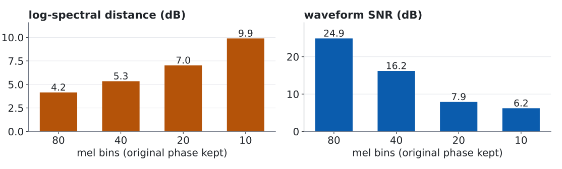
Demo 2. Keys 4, then a s d f. The phase is the original, so phase did not do it.

Two factors, pulled apart

Log-spectral distance from the original, in dB. Same utterance throughout.

Magnitude ╲ Phase	original	Griffin–Lim \times 256	random
linear	0.00	1.74	8.47
mel-80 → linear	4.38	6.35	9.07

• Read across a row: that is what phase costs
• Read down a column: that is what mel costs
• The old three-way demo — original, Griffin–Lim, random — only ever showed you the top row

A TTS system that predicts a mel-spectrogram and then runs Griffin–Lim lives in the bottom-middle cell. It pays both costs at once, and you cannot tell which one you are hearing.

A free preview: waveform SNR does not track what you hear

As Griffin–Lim iterates, the spectrum gets closer to the original and the sound gets better. The waveform SNR stays below 0 dB the whole time — the “noise” has more energy than the signal.

SNR compares waveforms sample by sample, so it is extremely sensitive to phase. The ear is not. A metric can be precise, well-defined, and measuring the wrong thing.

Misconception — “a vocoder exists to put the phase back”

That is one third of the job. A neural vocoder that takes a predicted mel-spectrogram has to do three things at once:

	What is wrong with the input	Kind of loss
1	no phase	algorithmic — the information is mostly there; finding it is hard
2	mel, not linear: fine structure above a few kHz is gone	informational — it must be invented plausibly
3	the mel was predicted, so it is over-smoothed — an average of many plausible outputs	statistical — it must be sharpened (W8)

Griffin–Lim addresses only the first, and only partly. That is why it sounds metallic even on a perfect magnitude, and why it was replaced — not because phase is unrecoverable.

The same idea, twice more this semester

W10 — enhancement by masking. A network predicts a mask and multiplies the noisy STFT by it. The result is a matrix that nobody checked for consistency. In general it is not the STFT of any signal, and the ISTFT quietly averages the contradiction away.

W8 — vocoders built on the inverse STFT. One family of neural vocoders predicts a magnitude and a phase for each frame, then applies a plain ISTFT. Predicting phase directly is awkward because phase wraps — -\pi and +\pi are the same angle but far apart as numbers — and much of the design is about getting around that.

“Is this matrix actually a spectrogram?” is a question you can now ask of any system that edits or generates in the time–frequency domain.

Above the segment

Prosody has three acoustic handles

Everything so far described segments: this vowel, that stop. Some properties stretch across many segments — hence suprasegmental.

Handle	What you measure	What it carries
F_0	rate of vocal-fold vibration, per frame	lexical tone, intonation, emphasis, emotion
duration	how long each segment lasts	stress, phrase boundaries, speaking rate, hesitation
energy	amplitude per frame	stress, emphasis, how a phrase trails off

When a later week says “prosody” — controlling it (W9), or using it to predict the end of a turn (W12) — it means these three curves and nothing more mysterious.

Misconception — “F_0 and pitch are the same thing”

	F_0	pitch
What it is	a physical quantity: the rate at which the vocal folds open and close	a perceptual quantity: how high a sound seems to a listener
Where it lives	in the signal	in the listener
When there is no voicing	undefined — there is nothing to measure	can still be perceived

Whisper has no F_0 at all. Listeners still hear a question as a question.

Algorithms estimate F_0. Papers often call the result “pitch”. When the two come apart — whisper, creaky voice, a missing fundamental on a telephone line — it matters which one was meant.

Cepstrum: pulling source and filter apart

After the log, source and filter add. The envelope varies slowly along the frequency axis; the harmonics ripple quickly. So take a Fourier transform of the log-spectrum and they land in different places:

c(n) = \mathrm{IDFT}\bigl\{\log|X(k)|\bigr\}

F_0 estimation fails in two characteristic ways

Three families of method: the cepstral peak, the autocorrelation peak, and refinements of autocorrelation such as YIN. All share the same two failure modes.

1. Octave error. A signal with period T also repeats every 2T. Pick the wrong peak and you report F_0/2 — or 2F_0
2. Voicing decision. Is there an F_0 in this frame at all? Every tracker hides a threshold

See it: tones, and then a question

Demo 1, third time. Watch the blue dots — that is the F_0 track.

1. One syllable, four tones: mā má mǎ mà
2. A short sentence as a statement. Then the same words as a question
3. Switch to narrowband (n): the harmonics fan out and close up as F_0 moves — the same information, seen a second way

Look for two things: does each tone keep its shape when the sentence becomes a question? And what happens to the last syllable?

Tone and intonation share one curve

In English, F_0 is almost entirely free to carry intonation — statement or question, emphasis, attitude. In Mandarin, Taiwanese and Hakka, F_0 is already taken by the words. Intonation has to ride on top.

• Taiwanese adds tone sandhi: a syllable’s tone changes with its position in the phrase
• One number per frame carries the word, the sentence type, the emphasis and the mood

Misconception — “the source is the speaker, the filter is the content”

Two counter-examples, one in each direction. You have now seen both on screen.

Claim	Counter-example	Where you saw it
“The filter carries what is said”	Vocal-tract length scales every formant — and it belongs to the speaker	Demo 1: a different speaker’s dot lands elsewhere for the same vowel
“The source carries who and how”	Lexical tone lives in F_0 — and it is content	Demo 1: mā / má / mǎ / mà

Source and filter are separate mechanisms. They are not separate kinds of information. Any method that “disentangles content from speaker” by splitting along this line is making an assumption — check it against your language.

Three predictions for later weeks

If F_0 carries words, methods that grew up on English may behave differently on Mandarin, Taiwanese and Hakka:

Week	The English-default statement	What it might mean for a tone language
W6	“Semantic tokens flatten the intonation; content survives”	Flattening F_0 may remove lexical content, not just expressiveness
W9	“Prosody control: move F_0 freely”	F_0 cannot move freely without changing the words
W12	“Falling pitch signals the end of a turn”	The final syllable’s own tone is mixed into that cue

These are predictions to check, not established results. Each is a possible project, and together they give concrete shape to the research gap from Week 1.

Same name, different features

“Log-mel” is not one thing

Two “80-dim log-mel” front-ends can differ in the mel scale (HTK, or Slaney — librosa’s default), the filter normalisation, power vs. magnitude, the log floor, dither, pre-emphasis, and how the result is normalised.

Feed a pretrained model features built with the wrong recipe and nothing crashes. It just gets quietly worse.

An experiment we have not run yet

Demo 3, as a plan. Same audio, same pretrained recogniser. Change only the front-end recipe — swap the mel scale, or drop the filter normalisation — and measure the word error rate.

Predict before anyone measures: does WER move a little, or a lot? Does it depend on which knob?

This is the first of the four questions from Week 1, in its most concrete form:

Is the input the same? Two papers that both report “80-dim log-mel, 25 ms / 10 ms” have not told you enough to know.

We will run it once the toolchain for this laptop is settled, and bring the numbers back.

SNR, and the metric W10 will use instead

\mathrm{SNR} = 10\log_{10}\frac{\lVert \mathbf{s} \rVert^2}{\lVert \mathbf{s} - \hat{\mathbf{s}} \rVert^2}

Segmental SNR computes this per short frame and averages the dB values, so a loud vowel cannot hide a ruined consonant.

Both punish any change of overall gain. Separation papers use a version that does not:

\mathrm{SI\text{-}SDR} = 10\log_{10}\frac{\lVert \alpha\mathbf{s} \rVert^2}{\lVert \alpha\mathbf{s} - \hat{\mathbf{s}} \rVert^2}, \qquad \alpha = \frac{\hat{\mathbf{s}}^{\top}\mathbf{s}}{\lVert \mathbf{s} \rVert^2}

\alpha\mathbf{s} is the projection of the estimate onto the reference: the \alpha that minimises \lVert \alpha\mathbf{s} - \hat{\mathbf{s}} \rVert^2 satisfies \alpha \lVert \mathbf{s} \rVert^2 = \hat{\mathbf{s}}^{\top}\mathbf{s}. Inner products and projections — for the third time today.

None of these predicts word error rate, and you have already heard why: they compare waveforms, and neither ears nor recognisers do.

Three ways to represent the same half second

	Size \times rate	Values	Where it comes from
log-mel	80 \times 100 Hz	continuous	fixed — today
SSL feature	hundreds \times\ 50 Hz	continuous	learned — W5
codec tokens	a few \times 12.5–50 Hz	discrete	learned, quantised — W6

What this week put on the three axes

Axis	What we now know
Representation	The spectrogram drops phase; mel drops fine detail. The first loss is algorithmic and recoverable. The second is informational and is not.
Latency	The hop sets the clock, \Delta = H / f_s. The window adds L/2 of lookahead. Every later stride slows the clock further.
Supervision	None. Every number today was chosen by a person — which is why “log-mel” is not one thing.

The front-end decides what every later layer is allowed to know. It is the cheapest part to compute, and the most expensive to get wrong.

Reading, and next week

Read this week

• Jurafsky & Martin, Speech and Language Processing, 3rd ed. draft, Ch 15 Phonetics and Speech Feature Extraction — both halves
• Huang, Acero & Hon, Spoken Language Processing, Ch 2, 5, 6 — if you want the derivations we skipped: cepstrum, LPC, source–filter

If one thing today was new to you, make it this one

• Griffin & Lim, Signal Estimation from Modified Short-Time Fourier Transform, IEEE Trans. ASSP, 1984 — short, readable, and the alternating-projection idea outlives the application

Next week — the alignment problem: from HMM to CTC

We have 100 frames per second. A sentence has perhaps a dozen phonemes per second. Nobody tells us which frames belong to which phoneme. That gap is the subject of Week 3.