A Systems View and the Latency Budget

Speech Processing & Human–Machine Interaction · Week 1

Hung-Shin Lee

Before anything else, listen

Two recordings. Same pre-recorded user, same benchmark task, same model family.

I will not tell you what to listen for yet.

Recording 1

Recording 2

The user started speaking at 9.6 s. The system did not stop.

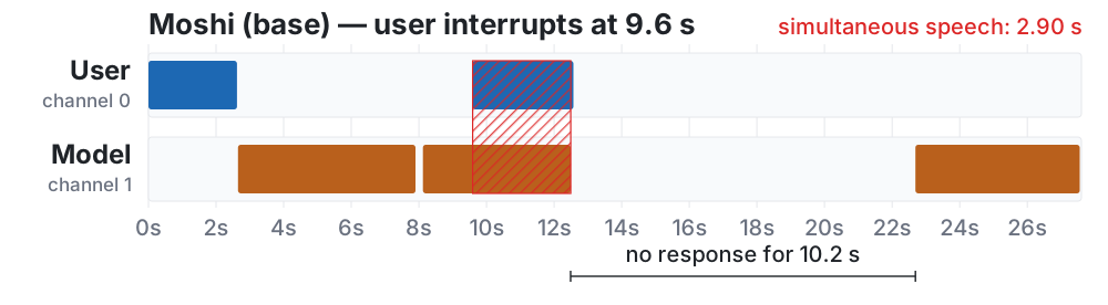
2.90 sthe model kept talking over the user

10.2 sthen said nothing at all

Same input, same architecture. Only the post-training differs.

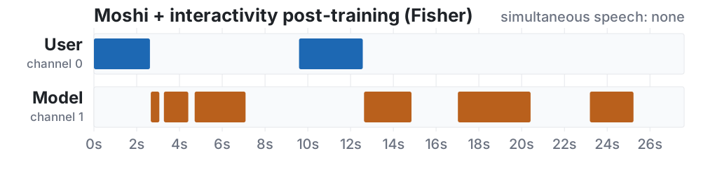
0.00 ssimultaneous speech

60 msfrom the user finishing to the model replying

Two opposite failures, one recording

A spoken dialogue system can fail by speaking when it should listen, and by staying silent when it should speak. Both happened in those 28 seconds.

Minimising response latency fixes the second failure and makes the first one worse.

This course is about the machinery that lets a system get both right at once — and about how to measure whether it did.

What this course is

By week 14 you should be able to build one of these, and to argue about it

Not “know about” — read the papers critically, measure the systems, defend design choices.

Part	Weeks	What it gives you
I — Foundations	W2–W6	front ends · alignment · streaming · SSL · neural codecs
II — Modules	W7–W10	ASR · TTS · controllability and evaluation · the front end
III — Dialogue	W11–W14	audio-native LMs · turn-taking · full duplex · evaluation

Fourteen weeks, and which week holds up which

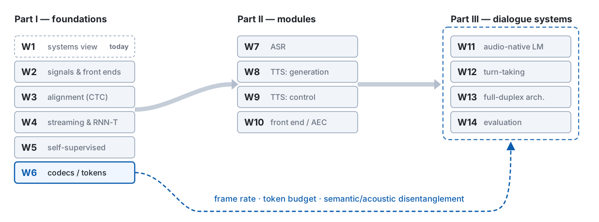
W6 is the hinge. If you skip one week, do not skip that one.

All of Part III rests on three ideas from W6:

• frame rate — tokens per second, and therefore decoder steps per second
• token budget — what a 30-minute conversation costs in context
• semantic / acoustic disentanglement — must meaning and timbre share one representation?

Every latency and quality ceiling downstream follows from how you turned speech into tokens.

What you should be able to do by the end of today

1. Draw the data flow of a cascade, an end-to-end speech-to-speech model, and a native full-duplex model — and point at the place where each one narrows the channel.
2. Decompose a target end-to-end latency into a per-module budget, say which entries are algorithmic delay and which are computational — and say what each entry actually measures.
3. Define half duplex versus full duplex operationally, and name four interaction behaviours a half-duplex system cannot have.
4. Argue, from human timing data, that turn-taking is prediction rather than detection — and therefore that a faster VAD does not solve it.
5. Interrogate a paper with four questions: is the input the same, how was the timing measured, what was normalised away, and what is the metric rewarding.

These five are the hooks that the next thirteen weeks attach to.

Three questions we ask every single week

Axis	The question
Representation	What representation does this layer use — waveform, spectrogram, continuous SSL feature, discrete token? What sets the frame rate?
Latency	How much of the budget does this module consume? Is that algorithmic delay (lookahead) or computational delay?
Supervision	Where does this capability come from — labels, self-supervision, synthetic data, or human preference?

These three are the coordinate system for the whole course. Slides in every later week come back to them.

Three architectures

From walkie-talkie to face to face

Walkie-talkie — one party at a time, and the handover has to be announced out loud.

Telephone — both channels are open the whole time, but people still take turns.

Face to face — speakers overlap, interrupt, hum agreement, and adjust a sentence while it is still coming out.

Spoken dialogue systems climbed this ladder in the same order. We are somewhere between the second rung and the third.

Where the metaphor breaks: two people talking are not two independent tracks that happen to overlap. Each is continuously adjusting to the other. That coupling is the hard part — and it is what W12 and W13 are about.

Cascade survives because every module can be debugged separately

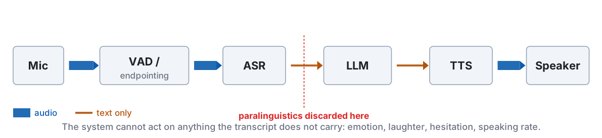
Thick line = audio. Thin line = text. The thickness is the information rate.

Everything the transcript cannot carry is gone at the ASR output

The LLM receives a string. Hesitation, amusement, shouting, speaking rate, whether the user had finished — and the timing of all of it — are gone.

A better ASR cannot fix this. The channel is simply too narrow for the signal. And note what a string has no field for at all: a clock.

Stop. What does a transcript throw away?

Write down everything you can think of. Two minutes.

emotion · laughter · sighs · hesitation and filled pauses · speaking rate · loudness · pitch range · accent and dialect · who is speaking · how many people are speaking · overlap · whether the utterance is finished · background environment · whether the speech is even addressed to the system

…and the one almost nobody writes down

The clock. When each word landed. How long that pause in the middle was. How long ago the user stopped.

A string has no timestamps. Not one.

End-to-end keeps the paralinguistics, and keeps text as a planning channel

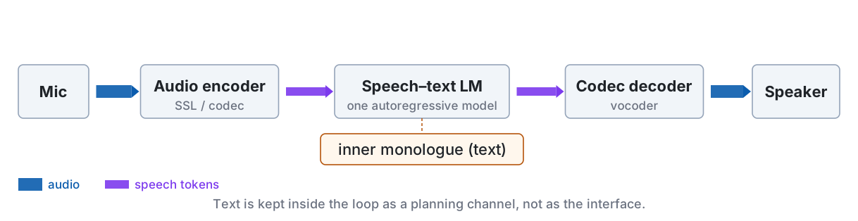
Nothing is forced through a transcript. But text does not disappear — it moves inside the model as an inner monologue.

What end-to-end costs

• Semantic degradation. Speech token sequences are one to two orders of magnitude longer than text for the same content. Training a language model on them erodes the language ability. [W11]
• Context cost. Frame rate × codebooks × conversation length. We will compute this in W6 and it is worse than people expect.
• Controllability and auditability. Tool calls, long-term memory, and “why did it say that” are all harder when there is no transcript to inspect.

The field’s current answer is neither pure cascade nor pure end-to-end. It is keeping text in the loop while never forcing audio through it.

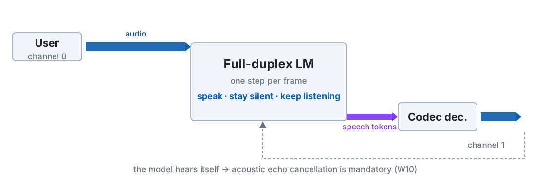
Full duplex is sequence modelling: silence is a token

y_t \;=\; f\!\left(x_{1:\,t+\ell},\; y_{1:\,t-1}\right), \qquad y_t \in \mathcal{V} \cup \{\varnothing\}

Once the model emits something every frame — including \varnothing, “say nothing” — turn-taking becomes ordinary next-token prediction.

Which failure can you afford?

	Cascade	End-to-end S2S	Native full duplex
Paralinguistics	lost at ASR output	preserved	preserved
Turn-taking	external VAD	external, usually	per frame
Semantic ability	full text LLM	degrades	degrades
Control, tools, audit	strongest	weaker	weakest today
Training cost	lowest	high	highest; needs two-track data
Debugging	per module	end to end only	end to end only

No ranking here — “end-to-end must be better” is a misconception. Pick the architecture whose failure mode your application can survive.

Misconception 1 — “full duplex means it supports interruption”

Interruption handling is a behaviour. It can be faked: detect user speech with a VAD, stop the TTS. That system is still half duplex.

The test is architectural: while the model is speaking, does the input stream still enter the computation and still change the next decision?

A VAD-gated cascade and a native full-duplex model can look identical on a clean interruption — and diverge completely on a mid-utterance pause, a backchannel, or two people talking.

The same test, drawn as two clocks

A VAD-gated cascade decides once — when the endpoint fires — and then plays a string. Between that decision and the external “stop”, x_t is not read and no y_t is chosen. Its output clock is broken; the frame clock of the model above it never stops.

The latency budget

Humans aim at a target, not at a minimum

Across 10 languages from 5 continents, informal conversation follows one norm: minimal gap, minimal overlap. Most turn transitions land near zero.

• Cross-language means differ by at most ±250 ms
• Responses that do not answer the question, or that go against its bias, come measurably later — and listeners read that delay as meaning

Delay is a signal, not just a cost. A system that always answers instantly is not maximally natural — it is uniformly ignoring one of the channels people use.

Misconception 2 — “lower latency is always better”

If a system answered every question in 40 ms, how would that feel?

Like it was not listening. Like it had prepared the answer before you finished. In human conversation, an instant response to a question that deserves thought is itself informative.

Remember Recording 2: 60 ms. Is that good? We genuinely do not know from the number alone — it depends on whether the content was worth 60 ms.

Humans answer faster than they can plan

Two numbers that do not fit together:

Quantity	Order of magnitude
Gap at a turn transition	clusters near zero — most transitions land within a couple of hundred ms
Planning one word for production	hundreds of ms before articulation even begins — call it 600 ms

If planning only started when the other person stopped, the earliest anyone could speak would be roughly 600 ms later. People do not take 600 ms.

So planning is already under way while the other person is still talking. The listener is predicting when the turn will end, and how. Turn-taking in humans is a prediction problem, not a detection problem.

Anything that only starts thinking after the user stops has already lost the race — and that is exactly what an endpoint threshold does.

Detection would reply 600 ms late. Prediction lands on time.

Put the two numbers on one axis and the conclusion is forced: the planning box has to start before the other speaker stops. Nothing else fits the observed gap.

Misconception 3 — “just make the VAD faster”

A VAD answers is someone speaking right now? — detection, answerable from the current frame.

Turn-taking asks is this person about to finish, and does what I just heard count as an interruption? — prediction, not answerable from the current frame at all.

Silence threshold	What you get
700 ms	safe, and the system feels slow
300 ms	fast, and it cuts people off mid-sentence
any value	one failure traded for the other

Tuning a threshold trades one failure for the other. It never creates the ability to predict, because a silence timer has no access to what was being said.

That is why W12 is about semantic endpointing — deciding from the words and the prosody, not from the length of the silence.

One sentence, two thresholds

The 500 ms pause inside the sentence and the silence after it are the same signal to a timer. Only the words tell them apart — and the timer never sees the words.

The budget we will refill every week

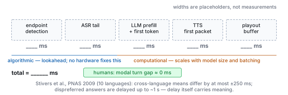
Two rules before you fill in a single cell

1 — Every cell holds only what happens after the user stops speaking.

Not the module’s total processing time. A streaming ASR has already consumed most of the utterance by the time the user stops; counting that work again inflates the whole budget by an order of magnitude. The ASR cell is the tail, not the transcription.

2 — This template is cascade-shaped.

A native full-duplex model has no endpoint-detection cell and no ASR tail. It emits on every frame, so there is nothing to wait for and nothing to flush.

In W13 this sheet will not fit the system we are studying. That failure is not a flaw in the sheet — it is the definition of full duplex, drawn in negative space.

Two kinds of delay, and only one of them is a hardware problem

A streaming model is a function that may peek \ell frames into the future:

\hat{y}_{1:t} \;=\; f\!\left(x_{1:\,t+\ell}\right)

\Delta frame shift (s) · \ell lookahead (frames) · n_{\text{layer}} layers · r_k right context of layer k · C chunk size (frames)

Algorithmic delay — still there on infinitely fast hardware:

D_{\text{alg}} \;=\; \underbrace{\ell\,\Delta}_{\text{lookahead}} \;+\; \underbrace{\alpha\,C\,\Delta}_{\text{waiting for the chunk}}, \qquad \ell \;=\; \sum_{k=1}^{n_{\text{layer}}} r_k, \qquad \alpha \in [\tfrac{1}{2},\,1]

Computational delay — the one you can buy your way out of:

D_{\text{comp}} \;=\; \mathrm{RTF}\cdot C\Delta \;+\; T_{\text{queue}}

Two claims hide in the first line: \ell is a sum, and \alpha is a range. The next two slides derive them.

Why \ell is a sum: right context stacks

Layer k at time t needs layer k-1 up to t + r_k. Apply that n_{\text{layer}} times:

t^{(k)} \;=\; t^{(k-1)} + r_k \qquad\Longrightarrow\qquad t^{(n_{\text{layer}})} \;=\; t + \sum_{k=1}^{n_{\text{layer}}} r_k \;=\; t + \ell

Why \alpha \in [\tfrac12, 1]: waiting for the chunk to fill

The user’s last frame lands at position j in its chunk and waits (C-1-j)\,\Delta. Averaged over where it lands:

\frac{1}{C}\sum_{j=0}^{C-1} (C-1-j)\,\Delta \;=\; \frac{C-1}{2}\,\Delta \;\approx\; \tfrac12\,C\Delta, \qquad\text{worst case } (C-1)\,\Delta \;\approx\; C\Delta

The mean is \alpha = \tfrac12; the tail is \alpha = 1. The p95 slide makes that distinction bite.

Add them up — every term after the user stops speaking

D_{\text{e2e}} \;=\; D_{\text{alg}} \;+\; D_{\text{comp}} \;+\; D_{\text{net}} \;+\; D_{\text{buf}}

Term	What it is	What moves it
D_{\text{alg}}	\ell\Delta + \alpha C\Delta	the model’s definition
D_{\text{comp}}	\mathrm{RTF}\cdot C\Delta + T_{\text{queue}}	hardware, model size, batching
D_{\text{net}}	round trip to wherever the model runs	deployment — on-device makes it zero
D_{\text{buf}}	audio held back so playback never stutters	the same buffer we meet again in the stop budget

A faster GPU moves exactly one of the four.

The arithmetic that eats the whole budget

A 15-layer encoder, each layer looking two frames to the right, at \Delta = 10 ms:

\ell \;=\; \sum_{k=1}^{15} r_k \;=\; 15 \times 2 \;=\; 30 \text{ frames} \qquad\Longrightarrow\qquad \ell\,\Delta \;=\; 30 \times 10\,\text{ms} \;=\; 300\,\text{ms}

With a chunk of C = 32 frames and \alpha = \tfrac{1}{2}:

D_{\text{alg}} \;=\; 300\,\text{ms} \;+\; \tfrac{1}{2}\times 32 \times 10\,\text{ms} \;=\; 300 + 160 \;=\; \mathbf{460\ \text{ms}}

A human-scale budget is a few hundred ms — gaps cluster near zero. We are at 460 ms before a single multiplication has happened — and D_{\text{comp}} has not been added yet.

The obvious counter-move — just shrink C — is the next slide.

Why not just shrink C?

Chunks arrive at 1/(C\Delta) per second; each is C queries against C+H keys (H = cached history):

\text{cost per second} \;\propto\; \frac{1}{C\Delta}\cdot C\,(C+H)\,d \;=\; \frac{(C+H)\,d}{\Delta}

Halving C halves the wait but removes only C from C+H: smaller chunks are more often and less efficient, not cheaper.

Misconception 4 — “latency is an engineering problem, not a research problem”

The streaming constraint does not sit on top of a model. It reaches inside and changes it.

• The loss function. RNN-T exists because an attention-based encoder–decoder cannot emit anything before it has seen the whole utterance. [W4]
• The representation. Low frame-rate neural codecs exist because decoder steps per second is a hard budget. [W6]
• The architecture. Causal masks and chunk-wise attention exist because the model is not allowed to look at the future. [W4, W8]

Each of those is a modelling decision forced by a timing requirement. Latency is not downstream of the research — it is one of its inputs.

The number that hurts is p95, not the mean

• Means add along a pipeline. Probabilities of being on time multiply: five modules each inside its own p95 leave the chain inside its budget only 0.95^5 \approx 77\% of the time (assuming independence).
• Averaging 320 ms but hitting 1.4 s twice a minute feels broken, not fast. Users experience the bad turns, not the distribution.

Report distributions. In W14 the goal becomes matching the human latency distribution with a distributional distance — not minimising a mean.

Before Demo 2: where does the time go after the user stops?

Why	The last ten slides built the budget on paper: every cell is time left after the user stops speaking, and some cells are a setting while others are compute. This demo fills the budget in from a real pipeline on this laptop.
What runs	One recorded Mandarin sentence with a pause in the middle (“I’d like a ticket to … Tainan, next Wednesday”) through a cascade: an energy-VAD endpoint, whisper.cpp, a local LLM (mlx-lm), a local TTS (mlx-audio). Every module boundary is time-stamped; ten runs, p50 and p95. Then, on headphones, a full-duplex model on the same laptop — listened to, not measured.
Watch for	Which cell is largest, how much each cell varies across the ten runs, and which of the two kinds of delay on p33 the largest one is. For the full-duplex model: when it talks, not what it says.

Live: measure your own pipeline

Demo 2. Prediction before we run it: which module will dominate?

The terminal fills in the budget sheet from p31 and draws the timeline; the end-to-end point on it is Recording 2 of the cold open, not this sentence.

Four behaviours a half-duplex system cannot have

The taxonomy

Behaviour	The user is…	The system must…	Week
Backchannel	still speaking; says “mm-hm”	recognise that no turn is being claimed, and keep going	W12
Interruption	taking the floor mid-answer	stop quickly, and keep what it had planned	W12, W13
Barge-in	speaking over the system’s own audio	separate its own voice from the user’s — AEC	W10
Overlap continuation	briefly overlapping, not taking the floor	continue rather than yield	W12
Proactive turn	silent	decide whether to open its mouth at all	open problem

Four of these five are out of reach for a half-duplex system. Interruption is the one it can fake — a VAD trigger that stops the TTS — which is exactly Misconception 1.

A base model can be a competent talker and a useless listener

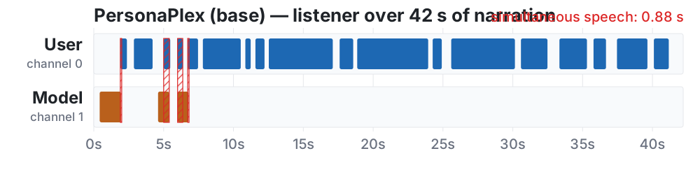
Forty-two seconds of narration. The model speaks three times, all within the first seven seconds, then nothing.

PersonaPlex (base) — first 20 s

The same model, post-trained: eleven short utterances spread across the whole clip

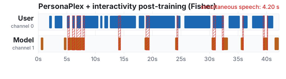
0.88 → 4.20 ssimultaneous speech

3 → 11model utterances, same 42 s

PersonaPlex + interactivity post-training — first 20 s

The same measurement is a defect in one task and a requirement in the other

Simultaneous speech: 2.90 s was the failure in Recording 1. 4.20 s was the improvement here.

There is no metric you can minimise to get good turn-taking. The target depends on what the user is doing — which means the system has to classify the situation before it decides.

The other budget: how long it takes to stop

The last section measured user stops → system starts. Interruption runs the other way.

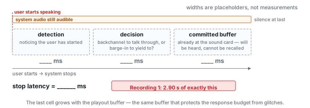
The third cell is the trap: a larger playout buffer protects you from glitches and makes you slower to shut up. One parameter, two faces — only one of them shows up in the usual latency number.

Misconception 5 — “the user should always win an interruption”

Interruptions have different functions: clarification, correction, agreement, seizing the floor. Yielding unconditionally means the system can never finish a necessary long answer — reading out an address, a dosage, a confirmation number.

“Always yield” is not politeness. It is a controllability failure, and it is measurable: W14’s benchmarks score both premature yielding and failure to yield.

And the cost of getting it wrong is now a number you can put on the sheet: every false yield costs one stop budget, committed buffer included.

Where we go from here

Each Part fills in part of the budget

Week	What it adds to the sheet
W2	frame shift — the smallest unit of delay there is
W4	lookahead and chunk size; ASR emission delay
W6	frame rate and token budget → decoder steps per second
W8	TTS first-packet latency; NFE versus quality
W10	AEC and front-end cost; why enhancement can raise WER
W13	per-frame decoding cost for a full-duplex model

Bring the sheet every week. By W14 you will have one diagram that explains where every millisecond of a spoken dialogue system goes.

Some of the gaps are yours to fill

Full-duplex research runs on two-track conversational recordings — one channel per speaker. English has corpora for this. Mandarin has some.

For Taiwanese Hokkien, Hakka and the Formosan languages, publicly available two-track dialogue data is close to non-existent — and the text side that interleaving depends on has no single settled orthography.

• The data does not exist, so even a small, well-designed corpus is a contribution.
• The orthography question is research, not preprocessing. [W6, W11]
• Almost nothing in Part III has been tested outside English and Mandarin.

When we reach W14’s open problems, this one has your name on it more than mine.

Four questions to ask of every paper in this course

1. Was the input the same? Today’s two recordings shared one pre-recorded user track, so the difference was attributable. Most system comparisons do not have that property.
2. How was the timing measured? Energy VAD, a reference VAD, forced alignment, or the model’s own logs? Our 2.90 s and 60 ms came from an energy VAD — the magnitudes hold, the milliseconds do not.
3. What was normalised away? WER depends on text normalisation; MOS depends on the rater pool and the scale anchors. Numbers from two different papers are usually not comparable at all.
4. What does the metric reward? A benchmark that scores only latency rewards a system that interrupts.

You will use these four every week — and they are also how you avoid writing a paper that someone else has to ask them about.

Next week, and what to read

W2 — Speech Signals, Auditory Front-Ends, and the Physics of Representation. The only systematic DSP week. Before the STFT it stops for a short refresher — inner products and projections — and then uses them three times.

If you read one thing this week:

• Lu et al., A Survey of Full-Duplex Spoken Dialogue Systems: Architectural Hierarchy, Interaction Ontology, and Decision State Machine, arXiv:2606.19453 (2026)

Two more, if you have time:

• Ji et al., WavChat: A Survey of Spoken Dialogue Models, arXiv:2411.13577 (2024) — the half-duplex era, for contrast
• Jurafsky & Martin, Speech and Language Processing, 3rd ed. draft (19 Aug 2026), Ch 26 — Conversation and its Structure

Sources

Audio and derived figures

Ohashi, Zeghidour, Défossez & Kharitonov, Multi-Faceted Interactivity Alignment in Full-Duplex Speech Models, EMNLP 2026 (arXiv:2606.11167). Samples: kyutai/interactivity-alignment-samples, licensed CC-BY-4.0. Clips were trimmed and re-encoded; timelines were computed from the released stereo WAVs.

Turn-taking timing

Stivers, Enfield, Brown, … Levinson, Universals and cultural variation in turn-taking in conversation, PNAS 106(26): 10587–10592, 2009.

Architecture taxonomy

Lu et al., arXiv:2606.19453 (2026).

Audio analysis code (energy VAD, overlap / response / stop latency, the two-track timeline): slides/scripts/analyze_duplex_audio.py, slides/scripts/make_duplex_timeline.py in the course repository.