From n-grams to Seq2Seq

NLP & Large Language Models · Week 1

Hung-Shin Lee

Five samples

Same corpus. Same prompt. One number changes.

225,333 words of Shakespeare. 14,560 distinct words. A word-level n-gram model, trained by counting.

Every sample below starts from the same seven words, and differs only in how many previous words the model is allowed to look at.

prompt … beside well in his person wrought To be …

Watch what happens to the output as that number goes up.

n = 1: the words are Shakespeare’s. Nothing else is.

n = 1　·　no context at all We than me or too: here separation PERDITA I majesty exhales the bring child have, night interchange, our to thereto and dad, kiss thinks a country’s the pedigree Thy For they Unless but,. the

• The unigram distribution is right: the, our, to appear at roughly the right rate
• Nothing else survives. No agreement, no syntax, no clause boundaries

A model of word frequency is a model of vocabulary, not of language.

n = 2: local fluency arrives. Global coherence does not.

n = 2　·　one word of context be to each of York, you might reproach your lordship cool your will show it. For thy due to your channel should be furnished with patience but a truth, seven night: He shift a word, my

• Two- and three-word spans are now plausible English: your lordship, furnished with patience
• Sentences still go nowhere. The model cannot remember what it said four words ago

One word of context buys local fluency. That is a remarkably good return on one word.

n = 4: this reads like Shakespeare.

n = 4　·　three words of context wrought To be set high in place, we did: he desires to make atonement Betwixt the Duke of York is there alive but we? And who durst mine when Warwick bent his brow? Lo, now my sovereign speaketh

• Clauses hold together. Rhetorical questions are well formed. Names are used consistently
• If I had not told you how this was produced, you might not have guessed counting

Four words of context, and pure counting, gets you something you would call fluent.

n = 8: this is not generation. This is recall.

n = 8　·　seven words of context well in his person wrought To be set high in place, we did commend To your remembrances: but you have found, Scaling his present bearing with his past, That he’s your fixed enemy, and revoke Your sudden approbation. BRUTUS: Say

That passage is in the training corpus, word for word, including the speaker tag that follows it.

Somewhere between n = 4 and n = 8, the model stopped generalizing and started remembering. Nothing in the training objective told us where that line was.

Two curves explain the whole sweep

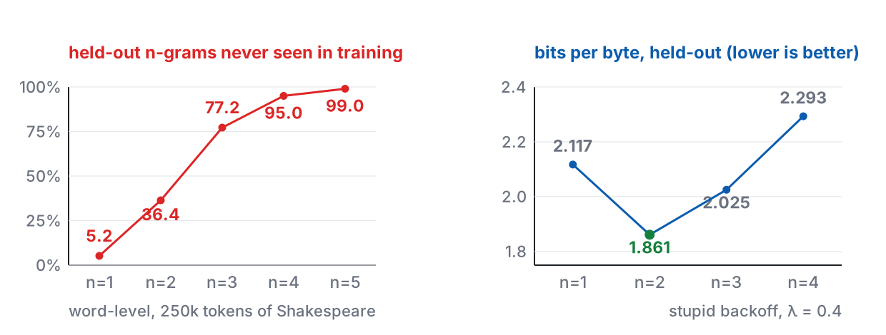
95.0%of held-out 4-grams never appeared in training

n = 2where bits-per-byte actually bottoms out

99.0%unseen at n = 5. More data will not fix this

Same prompt. A 2026 model. Live.

live · an open model on this laptop, the same seven words

Then one more, in Traditional Chinese, asking for something specific and checkable.

Third failure mode. Name it before I do.

• n = 1 failed locally: the words never combine
• n = 4 failed globally: every clause holds, the passage goes nowhere
• This one fails at neither scale — and will still state something checkable and wrong, in exactly the same even voice

Local, global, and fluent-but-false. The first two are solved problems. The third is why this course runs for fourteen weeks.

What this course is

By week 14 you should be able to open any layer and say why it is there

Not “what is a Transformer” — you can read that anywhere. The target is harder and more useful:

1. Derive the pieces: why 1/\sqrt{d_k}, why Chinchilla’s exponents, why DPO’s partition function cancels
2. Cost any design: given a model, say what it costs to train, to serve, and where the bottleneck actually is
3. Diagnose a failure: given a broken output, name the layer responsible and the mechanism
4. Judge a claim: read a 2026 paper and say whether its evidence supports its abstract

Every component in this course is introduced through the specific failure it was invented to fix.

Fourteen weeks, and which weeks hold up which

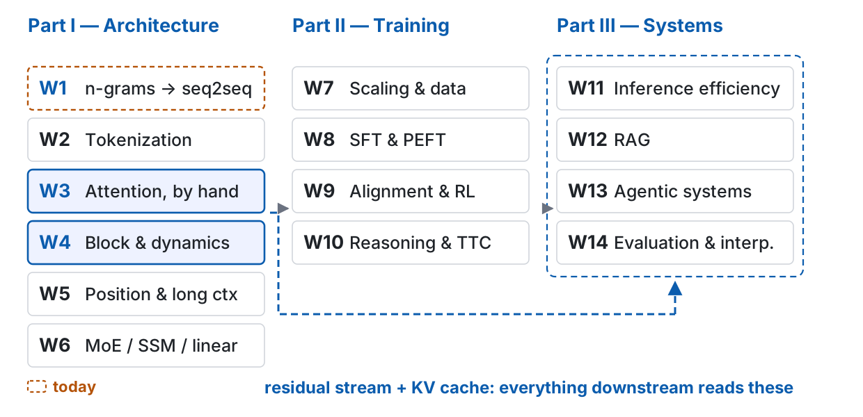
W3 and W4 are the hinge. If you skip one week, do not skip those two.

Everything in Part III reads from two objects built in W3–W4:

• the residual stream — a shared bus every layer reads from and writes back to
• the KV cache — the model’s actual state at inference time, and usually its dominant cost

By W11 the question is no longer “how does attention work” but “how many bytes does it move per token.” You cannot ask the second question until you have built the first.

What you should be able to do by the end of today

1. Write the n-gram MLE and the perplexity definition, and say why sparsity cannot be fixed by collecting more data
2. Explain how the distributional hypothesis becomes a loss function in word2vec, and where static embeddings structurally fail
3. Identify the gradient product in BPTT and the fixed-width bottleneck in seq2seq — and say which symptom Bahdanau attention was aimed at
4. State the equivalence between a language model and a compressor, using bits-per-byte, and say where that equivalence breaks

Item 4 is the one that carries furthest. It comes back in W7, W11 and W12.

The ledger we refill every week

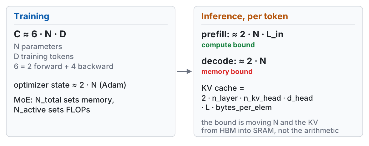
Two numbers, now, on paper

For a 7B dense model — work these out and keep them:

1. Training FLOPs at Chinchilla-optimal (D \approx 20N). Then: how many years on one consumer GPU — the 16 GB card your term project will actually run on?
2. The KV cache at batch 1, 32k context, FP16. Hold it against two real ceilings: that same 16 GB card, and the 64 GB of unified memory these demos run on.

Number 2 is the one that will surprise you. It is the shared motivation for W5, W6 and W11.

Capacity and bandwidth are different limits. 64 GB removes the first and does nothing at all about the second — which is most of W11, in one sentence.

Three questions we ask every single week

Axis	The question
Representation	What is the unit at this layer — byte, token, hidden state, KV entry, retrieved chunk, latent thought? Who chose it, and what does the choice cost downstream?
Compute	Does this spend training compute or inference compute? Is it FLOPs bound, or memory-bandwidth bound?
Supervision	Where does this capability come from? There are five possible answers — and today exactly one of them exists

The same observed behaviour can come from entirely different places on the third axis. That is the central dispute of W10 and W14.

Today, the third column has one entry

Where a capability can come from	today	arrives in
the pretraining distribution	✓	—
human demonstrations		W8
human preference		W9
a verifiable reward		W9 → W10
retrieved knowledge		W12
extra compute at test time		W10

Everything in today’s lecture — n-grams, word2vec, an LSTM language model, seq2seq — is self-supervised from raw text. Nothing else is on the menu yet.

W8 is where that column starts to branch. You will not feel how large that change is unless you notice how empty the column is today.

Four questions to ask of every paper in this course

1. Was the baseline actually tuned? The most common source of illusory progress. W8 and W9 both have cases where the gain vanishes after a learning-rate sweep
2. Is the comparison at equal compute? Iso-FLOPs, iso-parameter and iso-latency are three different comparisons, and they often disagree
3. What is the metric rewarding? In W11, KV-cache compression leaves perplexity almost untouched and quietly breaks instruction following
4. Is the claim mechanistic, or correlational? “The attention weight is high”, “the chain of thought wrote this step”, “the reward went up” — all three are correlations

You already used question 3 today: the n = 4 sample read best, and scored worse.

Practicalities

• Slides in English, taught in Mandarin. The speaker notes are mine and stay with me; the slides are yours, and they go up the same day
• There is an open-access English companion for the first three weeks: Zong, Zhao & Ma, NLP and Large Language Models (Springer / Tsinghua, 2026). Ch 5 is essentially today’s lecture in prose
• Assessed on two pieces of writing: a midterm report (40%) and a final paper (60%), both treated as conference submissions rather than coursework. Group work, plus two online discussions
• Everything is on the course site: weekly pages, the reading list, these slides, a half-life map saying which weeks go stale next year, and four Chinese guides for the two reports

hungshinlee.github.io/NLP-LLM

What you will run: nothing

Every demo in this course is run live, in front of you, on one laptop: 64 GB of unified memory, no CUDA.

• That buys room — a mid-sized model loads fine. It also rules things out: no vLLM, no bitsandbytes QLoRA, no FP8 or NVFP4 measurement
• When a demo cannot run on this machine, I will say so on the slide and we read the number out of the paper instead

That gap is not an apology. It is W11’s thesis arriving early: inference optimization is bound to hardware. Whether the same transformers code runs, and how fast, is the content of that week.

Your term project is a different machine: one 16 GB consumer GPU. Plan for that, not for what you see at the front of the room.

A language model is a compressor

Predicting well and compressing well are the same problem

Give me a distribution over the next token and I can build a code. Arithmetic coding reaches the entropy of that distribution, to within a bit.

H(p,q) = -\mathbb{E}_{x\sim p}\big[\log_2 q(x)\big] \quad\text{bits per symbol}

So the training objective of every model in this course is literally a compression rate.

This is the metaphor that runs the whole term. Pretraining is compression. A scaling law is the regularity in the compression ratio. Quantization compresses the compressor. RAG refuses to compress and looks things up instead.

Where the compression metaphor fails, and why that matters

What gets compressed is a distribution over strings, not a set of propositions.

The model can therefore emit a fluent string it never saw, that fits the distribution perfectly, and is false. That is not a bug in the compressor. That is what a compressor does.

• This is one mechanism behind hallucination — a mechanistic account, not a moral one
• It is also the reason W12 exists: if you need propositions with sources, do not compress them into weights
• And it is why “the model knows X” is a badly posed sentence. It has a distribution, not a knowledge base

Perplexity is not comparable across models

\mathrm{PPL} = \exp\!\left(-\frac{1}{T}\sum_{t=1}^{T} \log P(w_t \mid w_{<t})\right)

The denominator is T, the number of tokens — and that is a property of the tokenizer, not of the text.

The same Chinese paragraph can differ by more than a factor of two in T between two tokenizers. Perplexity moves with it.

Use bits-per-byte instead: total negative log-likelihood in bits, divided by the number of bytes. The denominator is a property of the text.

Live: the same paragraph, two tokenizers

One Traditional Chinese paragraph. Two open models whose tokenizers disagree sharply about Chinese. Identical text, identical bytes.

	model A	model B
tokens for the passage
perplexity
bits-per-byte

Predict before I run it: which rows disagree, and which row nearly agrees?

“Comparable” has three conditions

Bits-per-byte fixes the denominator. It does not make the number unconditional.

1. The tokenizer must be lossless on this text. One that normalizes away distinctions, or drops a rare character to UNK, never pays for those bytes — and therefore scores artificially low. For Traditional Chinese this is the easy mistake to make
2. The same bytes on both sides. Different held-out sets are different numbers, whatever the units
3. The same context length and document splitting. The same text scored with 8k of context beats itself at 2k, with no change to the model at all

“The only metric comparable across tokenizers” is a claim about the denominator. It is not a claim that the metric is immune to the evaluation setup.

And a low perplexity does not mean good generations

Even with the denominator fixed, likelihood and sample quality are largely independent in high dimensions. Theis, van den Oord & Bethge (2015) construct models that are good at one and bad at the other — in both directions.

You watched this happen forty minutes ago. The n = 4 sample read best of the four. It scored worse in bits-per-byte than n = 2.

• A model can put its mass in roughly the right place and still generate nothing you would keep
• And a model can generate beautifully by copying, while assigning poor probability to text it has never seen — which is exactly what n = 8 does

From counting to sharing parameters

Smoothing is not a hack. It is a statistical necessity.

The MLE is just a count ratio:

P(w_t \mid w_{t-n+1:t-1}) = \frac{C(w_{t-n+1:t})}{C(w_{t-n+1:t-1})}

With vocabulary V, there are V^n possible n-grams. Ours: V = 14{,}560, so V^4 \approx 4.5\times10^{16} — against 225,333 training words.

Good–Turing puts the total probability of everything unseen at roughly N_1/D, where N_1 counts the n-grams seen exactly once.

The MLE assigns zero to 95% of the 4-grams you will actually meet. Any usable model must therefore invent probability mass — and how it invents it is an inductive bias, not an implementation detail.

More data does not fix this

Doubling the corpus halves neither of these numbers by much. The count table grows; the space it must cover grows faster.

	n = 1	n = 2	n = 3	n = 4	n = 5
Unseen in held-out	5.2%	36.4%	77.2%	95.0%	99.0%
Distinct n-grams stored	13.7k	94.8k	182k	213k	222k

Notice the second row saturating: past n = 3, almost every new n-gram is seen exactly once. The table is memorizing, not estimating.

Counting cannot generalize to unseen contexts, because it has no notion that two contexts might be similar.

Why more data cannot fix it: Zipf and Heaps

V^n tells you the space is huge. It does not yet tell you that more data fails — the space is fixed while the corpus can keep growing. What closes that gap is the shape of the word distribution.

• Zipf: word frequency follows a power law. Most distinct types live in the tail
• Heaps: distinct types grow as |V| \propto D^{\beta}, \beta < 1 — sublinear, and yet never saturating
• So the share of hapax does not fade away as D grows. Put that into Good–Turing’s unseen mass, \approx N_1/D:

The probability mass sitting on things you have never seen does not go to zero as the corpus grows. Sparsity is a property of language, not a shortage of text.

Two inductive biases for one problem

	n-gram	Neural LM (Bengio 2003)
What it stores	a table of counts	a parameterized function
Unseen context	zero, then a backoff rule	interpolates in a continuous space
Similarity	none; strings are atomic	built in; nearby vectors behave alike
Cost of more context	table size grows like V^n	a few more input weights

The move from 2003 onwards was not “neural networks are stronger”. It was replacing a lookup table with a function, so that unseen inputs land somewhere sensible. Everything after this — including attention — is a variation on how to build that function.

So “an LLM is just a bigger n-gram” is wrong in both directions: the inductive bias is different, and at the long tail an LLM does fall back on memorization — which is exactly what we watched happen at n = 8.

Where does the n = 8 sample sit on that table?

It was fluent. It was grammatical. It was, word for word, in the training set.

Ask it of any model, at any scale:

• Is this output interpolation — a point in a continuous space the model has never visited?
• Or is it retrieval — a path through the training data that happens to be smooth?

For a 4-gram table you can check by grepping the corpus. For a model trained on ten trillion tokens you cannot. W14 is about what we do instead.

The distributional hypothesis, and its trap

The hypothesis becomes a loss function

You shall know a word by the company it keeps. Word2vec (SGNS) turns that into an objective:

\mathcal{L} = -\log\sigma(\mathbf{u}_o^\top \mathbf{v}_c) \;-\; \sum_{k=1}^{K}\log\sigma(-\mathbf{u}_k^\top \mathbf{v}_c)

Push a word and its true context together; push it away from K sampled non-contexts.

Read the second term carefully. The set of negatives defines what “similar” is going to mean. Change the negative sampling and you change the geometry.

Live: the nearest neighbour of love in this corpus

PPMI on a 4-word window, then SVD to 200 dimensions, on the same Shakespeare. Function words removed for display.

query	nearest neighbours (cosine)
love	hate .412 · know .405 · him .405 · devotion .394 · romeo .381
king	richard .781 · edward .666 · iii .642 · vi .630 · ii .625
father	child .511 · son .507 · york .475 · heir .465 · grandfather .458

The nearest neighbour of love is hate.

Antonyms beat synonyms

	pair	cosine
antonym	love / hate	0.412
antonym	life / death	0.404
antonym	good / bad	0.228
antonym	friend / enemy	0.220
synonym	good / excellent	0.212
synonym	sword / blade	0.163

Both synonym pairs score below every antonym pair. If cosine measured semantic similarity, this table would be impossible.

This is not a word2vec quirk

Levy & Goldberg (2014): SGNS is implicitly factorizing a shifted PMI matrix. That is why the demo above — PPMI plus a truncated SVD — reproduces the same behaviour, and why the behaviour is a property of the objective, not of the optimizer.

Cosine similarity means “similar under the notion of similarity this model’s training objective defines.” Nothing more. Say that sentence out loud whenever you see a cosine on a slide.

• Static embeddings additionally fail on polysemy: one vector per word, so bank gets one point for two senses
• W3 fixes polysemy — contextual representations — and does not fix the cosine problem

Why recurrence died

The gradient is a product, and products go to zero

\frac{\partial \mathcal{L}}{\partial h_1} = \frac{\partial \mathcal{L}}{\partial h_T}\prod_{t=2}^{T}\frac{\partial h_t}{\partial h_{t-1}}

T factors multiplied together. Spectral radius below 1 and it vanishes; above 1 and it explodes. Either way, the effective memory is far shorter than the sequence.

An LSTM’s gates replace part of that multiplicative path with an additive one — the cell state is carried forward and added to, not repeatedly transformed.

Remember the phrase additive path. In W4 the same trick reappears under a different name — the residual stream — and it is the reason 100-layer models train at all.

Then seq2seq squeezed everything through one vector

Encoder reads the whole source, produces one fixed-width vector, decoder writes from it.

A 5-word sentence and a 50-word sentence get the same number of floats. Translation quality fell off with length, and it fell off exactly the way a fixed-capacity channel predicts.

Bahdanau, Cho & Bengio (2015) aimed at that one symptom:

c_t = \sum_i \alpha_{ti} h_i, \qquad \alpha_{ti} = \mathrm{softmax}_i\big(a(s_{t-1}, h_i)\big)

Instead of one vector, let the decoder build a different weighted read of the source at every output step.

That attention is cross-attention, not self-attention

The query is the decoder state s_{t-1}. The keys and values are the encoder states h_i. Query and key/value come from two different sequences.

Self-attention — one sequence attending to itself — does not appear until 2017.

Keep these apart or W5 will not make sense. “Why does the model need extra position information?” is a question that only arises once a sequence attends to itself. A decoder already runs in time order; an encoder–decoder alignment never needed to be told what came first.

• W3’s causal mask is a statement about self-attention. It has no counterpart here
• The weights \alpha_{ti} do look like an alignment, and that resemblance is where a decade of misreading begins — W3

Attention is older than the Transformer

Bahdanau attention is 2015. The Transformer is 2017. What 2017 removed was recurrence, not attention.

“Attention Is All You Need” is a claim about what you can delete, not about what was invented.

Two consequences you need today:

• Once recurrence is gone, nothing in the architecture knows word order any more — hence positional encoding, and hence W5
• Once recurrence is gone, the sequence dimension is fully parallel — and that is the actual cause of death

RNNs did not lose on quality. They lost on throughput.

An RNN’s hidden state at step t requires step t-1. The sequence dimension cannot be parallelized. So you cannot spend more GPUs to train on more data, and after 2017 that was the only thing that mattered.

This is the single most important sentence in today’s lecture for understanding the rest of the course.

And what recurrence never lost

At inference an RNN carries a fixed-size state. A Transformer carries a KV cache that grows with every token it generates.

So the trade was narrower than the usual story: recurrence lost training throughput, and kept its inference advantage the whole time.

Which is why, in 2026, recurrence is back — Mamba, gated linear attention, the hybrid architectures of W6. What changed is not the recurrence. Someone solved the training half, and the advantage that had been sitting on the other side all along became collectable.

Where this goes

Each Part fills in part of the ledger

Part	What it adds to the compute ledger
I — Architecture	where the FLOPs and the bytes actually go; what the unit of representation is at each layer, and who chose it
II — Training	how to spend a training budget optimally, and what post-training buys that pretraining cannot
III — Systems	why decode is memory bound; what a retrieval hop costs; and how we find out whether any of it works

Today you built the first row of that ledger with a model you could have written in twenty lines.

Next week: the unit you cannot change after training

Tokenization. The one design decision in the whole system that cannot be fixed post hoc.

• We will build BPE by hand, and put the same Traditional Chinese paragraph through five tokenizers to measure fertility
• Perplexity comes back — this time with the actual token counts that make it incomparable
• And a 2026 result: the tokenizer shifts the compute-optimal parameter/data configuration, which moves it out of preprocessing and into architecture

Before then, read: JM3 Vol I ch 2 Words and Tokens (the 2026-08-19 release — pin that one), and ZZM ch 7, which covers the same ground with Chinese segmentation in it and is open access. To review today: ZZM ch 5 and ch 3.

Nothing to install. Every demo in this course runs at the front of the room.

Sources

Textbooks · Jurafsky & Martin, Speech and Language Processing, 3rd ed., 2026-08-19 draft release — ch 2 Words and Tokens, ch 3 N-gram Language Models, ch 5 Embeddings, ch 14 RNNs and LSTMs · Zong, Zhao & Ma, Natural Language Processing and Large Language Models, Springer Nature Singapore / Tsinghua University Press, 2026 (open access) — ch 5 Basic Language Models, ch 3 Distributed Representation, ch 4 Sequence Generation Models, ch 2.5 RNN and LSTM

Papers · Bengio, Ducharme, Vincent & Jauvin, A Neural Probabilistic Language Model, JMLR 2003 · Mikolov, Chen, Corrado & Dean, Efficient Estimation of Word Representations in Vector Space, arXiv:1301.3781 · Mikolov, Sutskever, Chen, Corrado & Dean, Distributed Representations of Words and Phrases and their Compositionality, NeurIPS 2013 · Levy & Goldberg, Neural Word Embedding as Implicit Matrix Factorization, NeurIPS 2014 · Sutskever, Vinyals & Le, Sequence to Sequence Learning with Neural Networks, NeurIPS 2014 · Bahdanau, Cho & Bengio, Neural Machine Translation by Jointly Learning to Align and Translate, ICLR 2015 (arXiv:1409.0473) · Vaswani et al., Attention Is All You Need, NeurIPS 2017

Papers, on today’s two framing claims · Bengio, Simard & Frasconi, Learning Long-Term Dependencies with Gradient Descent is Difficult, IEEE Transactions on Neural Networks 5(2):157–166, 1994 — the multiplied-gradient argument · Hochreiter & Schmidhuber, Long Short-Term Memory, Neural Computation 9(8):1735–1780, 1997 — the additive path · Delétang, Ruoss, Duquenne, Catt, Genewein, Mattern, Grau-Moya, Wenliang, Aitchison, Orseau, Hutter & Veness, Language Modeling Is Compression, arXiv:2309.10668 (2023) — compression as a measurement, not only a metaphor · Theis, van den Oord & Bethge, A note on the evaluation of generative models, arXiv:1511.01844 (2015) — why a low perplexity does not mean good samples

Data and figures · Corpus: the standard tinyshakespeare split of Shakespeare’s works (public domain). All n-gram generations, sparsity percentages, bits-per-byte values, cosine similarities and nearest-neighbour lists on these slides were computed for this course by scripts/make_demo_w01.py; the figures by scripts/make_figs_w01.py. Nothing on these slides is a remembered number.

Search terms, not citations · arithmetic coding neural language model · bits per byte evaluation · Chen & Goodman empirical study of smoothing · Zipf Heaps law vocabulary growth · attention is not not explanation